SamplePublisher`GrassmannCalculus`
NewtonianGravitationalDynamics |
|
| | ||||
Details and Options
Examples
(1)
Basic Examples
(1)
In[1]:=
<<GrassmannCalculus`
The following brings up a form for data entry.
Global data:
Gravitational constant
Two or Three dimensional coordinates
Number of objects- 2 to 5
The following brings up a form to enter
For each object:
Mass
Initial position
Initial velocity
Global data:
Gravitational constant
Two or Three dimensional coordinates
Number of objects- 2 to 5
The following brings up a form to enter
For each object:
Mass
Initial position
Initial velocity
The following is an example with units for the earth's orbit about the sun.
In[2]:=
earthSunData=
[];
NewtonianGravitationalDynamics |
The following preserves the data that was entered.
In[3]:=
sampleData=
Earth Orbit with Units
;The result is an Association with the following Keys.
In[4]:=
Keys[sampleData]//FullForm
Out[4]//FullForm=
List["objects","coordinates","G","objectForceRules","forcePairRules","objectForces","basicEquations","basicGravitationalEquations","consolidatedObjectRules","gravitationalEquationsWithData","solveVariables","p1","p2"]
We won't show all of the data here. The equations to be solved with the data are extracted with:
In[5]:=
sampleData["gravitationalEquationsWithData"]
Out[5]=
[t]+,v[p1][x][t][t],v[p1][x][0]0,x[p1][0]0,[t]+,v[p1][y][t][t],v[p1][y][0],y[p1][0]0,[t]+,v[p2][x][t][t],v[p2][x][0]0,x[p2][0],[t]+,v[p2][y][t][t],v[p2][y][0],y[p2][0]0
′
v[p1][x]
x[p1][t]
-1
M
G
3/2
(+)
2
(-x[p1][t]+x[p2][t])
2
(-y[p1][t]+y[p2][t])
x[p2][t]
1
M
G
3/2
(+)
2
(-x[p1][t]+x[p2][t])
2
(-y[p1][t]+y[p2][t])
′
x[p1]
′
v[p1][y]
y[p1][t]
-1
M
G
3/2
(+)
2
(-x[p1][t]+x[p2][t])
2
(-y[p1][t]+y[p2][t])
y[p2][t]
1
M
G
3/2
(+)
2
(-x[p1][t]+x[p2][t])
2
(-y[p1][t]+y[p2][t])
′
y[p1]
-0.090975
m/s
′
v[p2][x]
x[p1][t]
1
M
☉
G
3/2
(+)
2
(-x[p1][t]+x[p2][t])
2
(-y[p1][t]+y[p2][t])
x[p2][t]
-1
M
☉
G
3/2
(+)
2
(-x[p1][t]+x[p2][t])
2
(-y[p1][t]+y[p2][t])
′
x[p2]
0.983236
au
′
v[p2][y]
y[p1][t]
1
M
☉
G
3/2
(+)
2
(-x[p1][t]+x[p2][t])
2
(-y[p1][t]+y[p2][t])
y[p2][t]
-1
M
☉
G
3/2
(+)
2
(-x[p1][t]+x[p2][t])
2
(-y[p1][t]+y[p2][t])
′
y[p2]
6.38529
au/yr
The variables to be solved for are:
In[6]:=
sampleData["solveVariables"]
Out[6]=
{x[p1],v[p1][x],y[p1],v[p1][y],x[p2],v[p2][x],y[p2],v[p2][y]}
This system is solved in Lecture 4 of The Theoretical Next Step. It involves using the UnitsHelper package to obtain unit free numerical equations.
It's possible to enter symbolic values for the parameters and then substitute for them later.
The following is a pure numeric case.
In[7]:=
symbolicData=
[];
NewtonianGravitationalDynamics |
In[8]:=
sampleData2=
Numeric Case
;In[9]:=
solutions=NDSolve[sampleData2["gravitationalEquationsWithData"],sampleData2["solveVariables"],{t,0,1}]
Out[9]=
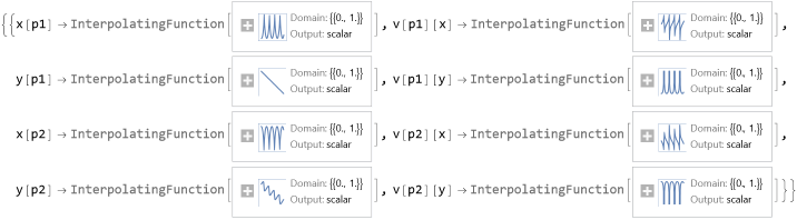
In[10]:=
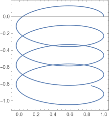
ParametricPlot[{x[p2][t],y[p2][t]}/.solutions,{t,0,1},PlotRangeAll,FrameTrue]
Out[10]=
 |
|
 |
|
""