In[]:=
(*deployswithcanonicalname*)deploy
Sat 25 Nov 2023 13:10:21
2-NN<>Least Squares
2-NN<>Least Squares
High level experiments relating to least squares optimization/NN.
Companion to “2-NN<>Least Squares” notability
Previous version: nn<>least-squares.nb
Blog-trajectories doc
Rough (transient) prototyping on nn-least-squares-scratch3.nb
Dropbox version history: git0/nn-linear
Companion to “2-NN<>Least Squares” notability
Previous version: nn<>least-squares.nb
Blog-trajectories doc
Rough (transient) prototyping on nn-least-squares-scratch3.nb
Dropbox version history: git0/nn-linear
Alpha Capacity, Effective Rank, Power-law decay
Alpha Capacity, Effective Rank, Power-law decay
Exp approximation of power
Exp approximation of power
In[]:=
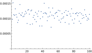
eval:=(d=100;X=RandomReal[{-1,1},{d,d}];H=X.X;H=H/Norm[H];A=-H;t=10;ii=IdentityMatrix[d];traceNormalize[vec_]:=vec/Total[vec];u=traceNormalize@RandomReal[{0,1},{d}];v=traceNormalize@RandomReal[{0,1},{d}];Clear[f];u=traceNormalize@ConstantArray[1.,{d}];v=u;f[mat_]:=u.mat.v;f@MatrixExp[tA]-f@MatrixPower[ii+A,t]);ListPlot@Table[eval,{100}]
Out[]=
In[]:=
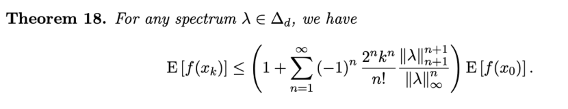
With[{t=-3},LogPlot[{Exp[tx],(1+x)^t},{x,-1,1},PlotLegends->{"exp","power"}]]
Out[]=
In[]:=
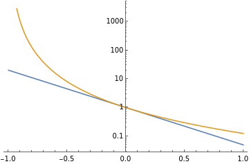
d=3;X=RandomReal[{-1,1},{d,d}];H=X.X;H=H/Norm[H];H=DiagonalMatrix[{1,1/2,1/3}];A=-H;t=10;ii=IdentityMatrix[d];LogPlot[{Tr@MatrixExp[tA],d+tTr[A],Exp[t*Max@Eigenvalues@A]},{t,0,d*d},PlotLegends->{"true","linear","exp"}]
Out[]=
In[]:=
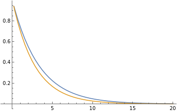
With[{x=.3},Plot[{Exp[-tx],(1-x)^t},{t,-1,20},PlotLegends->{"","(1-x"}]]
-xt
e
t
)\),
Out[]=
In[]:=
Clear[n];GeneratingFunction[,n,x]
n
a
Out[]=
1
1-ax
Incomplete Gamma result
Incomplete Gamma result
Loss of power-law decay in the continuous/continuous limit

Exp polynomial Factoring
Exp polynomial Factoring
Differential equation approach
Differential equation approach
Continuous GD with p-decay
Continuous GD with p-decay
Continuous GD + SGD
Continuous GD + SGD
Kolmogorov Concentration
Kolmogorov Concentration
d=1000;p=1.;h$=Table[,{i,1,d}];updateDet[e_]:=*e;genTraj[e0_]:=NestList[updateDet,e0,10000];B=10;randomTrajectories=genTraj/@RandomVariate[NormalDistribution[],{B,d}];norm2[point_]:=point.point;plot1=ListLinePlot[Map[norm2,randomTrajectories,{2}],ScalingFunctions->"Log",PlotStyle->Directive[Gray,Opacity[.2]]];e0=N[
-p
i
2
(1.-h$)
d
]~Join~ConstantArray[0,d-1];nonRandom=genTraj/@{RotateLeft[e0],RotateRight[e0]};plot2=ListLinePlot[Map[norm2,nonRandom,{2}],ScalingFunctions->"Log"];Show[plot1,plot2]Free probability
Effective rank:
- Nov 24: ask stats.SE “Frobenius norm of a product of Gaussian matrices” post
Shared notebooks:
- purity-of-matrix-products.nb (Mathoverflow post, my own answer)
- Frobenius norm of product of random matrices
- sent to Thomas thomas-convergence-of-rank.nb
- forum-burda-evals.nb (checking for commutativity)
- forum-product-of-matrices.nb
- Formulas-contents/”dot product formulas” notability, “NN<>Least Squares:Frobenius/Trace/Rank” notability
- formula-check.nb
- scicomp (Effective algorithm): https://scicomp.stackexchange.com/questions/43039/estimating-the-sum-of-4th-powers-of-singular-values/43044#43044
- fast effective rank https://www.wolframcloud.com/obj/yaroslavvb/nn-linear/forum-sum-of-singular-vals.nb
3.59-3.60 of https://arxiv.org/pdf/1510.06128.pdf
Also https://iopscience.iop.org/article/10.1088/1742-6596/473/1/012002/pdf
forum-burda-evals.nb
Also https://iopscience.iop.org/article/10.1088/1742-6596/473/1/012002/pdf
forum-burda-evals.nb
Construct MeijerG:
1/n
1/n
Moments of Fuchs-Catalan density
Moments of Fuchs-Catalan density
Gaussian matrix moments
Gaussian matrix moments
Solve using S-transform
Solve using S-transform
Now for squared Wishart
Simplified solving using S-transform
Simplified solving using S-transform
Convergence of effective rank
Convergence of effective rank
Isometry/Ahle
Isometry/Ahle
TLDR; information is kept on isometries, but isometry + small noise will lose it
TODO: learning rates complete picture
TODO: learning rates complete picture
For a given problem, we have following variables
Step size: 1/Tr, optimal
Batch size: b=1, b=inf
Norm for alpha=1: l1, l2, linf
Norm for alpha=opt: l1, l2, linf
Growth at C=I: l1, l2, linf
Growth at C=stationary: l1, l2, linf (should be same as norm for l2)
Refactor these by using common methods. Get graphs for Gaussian with infinite size, Gaussian with d=1000, MNIST, MNIST whitened
Questions
Questions
Is stationary distribution/stationary more representative for GD than for SGD?
Compare behavior at steps=d for common distributions
Compare behavior at steps=d for common distributions