In[]:=
Thu 6 Apr 2023 14:16:57
High level experiments relating to least squares optimization/NN’s summarized here.
More specific notebooks
gd-vs-sgd: shared code for running spectra analysis
linear-estimation-*: shared code for gradient descent/learning rate finders
nn<>least-squares-scratch: unorganized pre code
More specific notebooks
gd-vs-sgd: shared code for running spectra analysis
linear-estimation-*: shared code for gradient descent/learning rate finders
nn<>least-squares-scratch: unorganized pre code
Utilities
Utilities
Step length after normalization
Step length after normalization
Break - even for small batches
Break - even for small batches
Get GS length dependence on batch size
Get GS length dependence on batch size
Get residual dependence on batch size
Get residual dependence on batch size
Decay of GS contributions
Decay of GS contributions
Growth of singular values squared (linear)
Growth of singular values squared (linear)
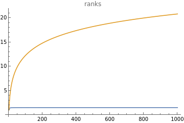
Convergence of effective rank
Convergence of effective rank
Improvement from average Kaczmarz step
Improvement from average Kaczmarz step
Ortho decay and effective rank?
Ortho decay and effective rank?
Preconditioner improvements
Preconditioner improvements
Stable rank, effective dimension, required sketch size
Stable rank, effective dimension, required sketch size
Decay of eigenvalues vs Cholesky vs Pivoted
Decay of eigenvalues vs Cholesky vs Pivoted
Does stable rank predict largest usable batch size?
Does stable rank predict largest usable batch size?
What is the norm of typical batch at size=stable rank?
What is the norm of typical batch at size=stable rank?
How angle and stable rank relate for X with 2 stacked rows
How angle and stable rank relate for X with 2 stacked rows
Normalization and efficiency for various distr?
Normalization and efficiency for various distr?
Optimal vs average optimal step
Optimal vs average optimal step
Expected drop as a function of dimension
Expected drop as a function of dimension
Expected drop as cross correlation
Expected drop as cross correlation
Harmonic mean of sensitive rank
Harmonic mean of sensitive rank
Estimating Frobenius norm
Estimating Frobenius norm
Step sizes for power law decay
Step sizes for power law decay
Use Gaussian identities to estimate step sizes
Use Gaussian identities to estimate step sizes
Effective ranks and norm growth
Effective ranks and norm growth
Harmonic interpolation of step sizes
Harmonic interpolation of step sizes
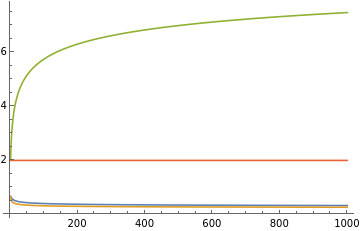
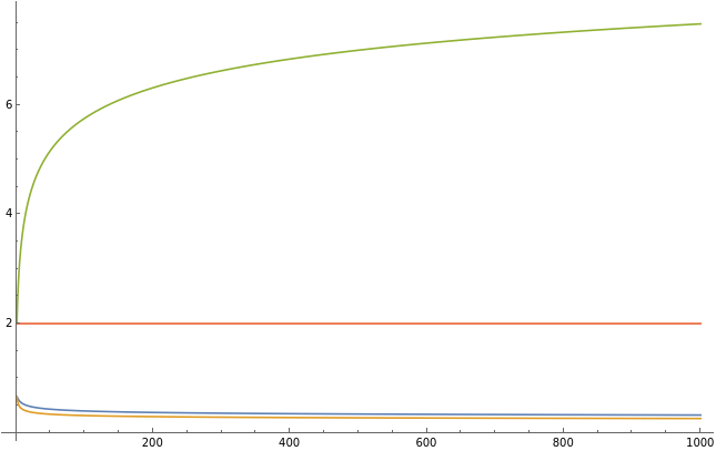
Deterministic vs stochastic rates
Deterministic vs stochastic rates
Deterministic gradient learning rates goes up with dimension, stochastic learning rate goes down. Huge difference in learning rate in deterministic case, tiny difference for stochastic case.
In[]:=
maxBatch=50;batchSizes=First/@Partition[Range[maxBatch],Max[1,Floor[maxBatch/10]]];evals=N@Table[,{i,1,d}];trSigma=Total[evals];trSigma2=Total[evals*evals];normSigma=Max[evals];estimateR1[X_]:=With{sigma=X.X},;estimateR2[X_]:=With{sigma=X.X},;getRates[evals_]:=trSigma=Total[evals];trSigma2=Total[evals*evals];normSigma=Max[evals]; ,,2,,,;decay=1.1;vals=Transpose@Table[getRates[N@Table[,{i,1,d}]],{d,1,1000}];ListLinePlot[vals[[;;4]],PlotLegends->{"stochastic first","stochastic anytime","determistic first","deterministic anytime"}]ListLinePlot[vals[[5;;]],PlotLegends->{"r","R"},PlotLabel->"ranks"]
-decay
i
2
Norm[X,"Frobenius"]
Norm[sigma]
2
2
Norm[X,"Frobenius"]
Norm[sigma,"Frobenius"]
2trSigma
2trSigma2+
2
trSigma
2
2normSigma+trSigma
trSigma
trSigma2
2
normSigma
trSigma2
normSigma
2
trSigma
trSigma2
-decay
i

Out[]=
Out[]=
Out[]=
Formula for loss decay on power law
Formula for loss decay on power law