MinEccentricityConics Explored
MinEccentricityConics Explored
Lyle Ramshaw, lyle.ramshaw@gmail.com
Introduction
Introduction
Given control points , , and in the plane, consider arcs of conics that are inscribed in the triangle in the sense that they start at , heading toward , and end at , heading away from . There is a one-parameter family of such inscribed conic arcs. Here are some of the arcs in one such family.
P
Q
R
△PQR
P
Q
R
Q
(Two coding remarks: We write the points , , and in Mathematica code as , , and ; and the following assignment is for later Manipulates.)
P
Q
R
p
q
r
In[]:=
savingDefinitions=True
Out[]=
True
In[]:=
With[{p={-2,0},q={0,3},r={3,-1}},Graphics[{Table[BSplineCurve[{p,q,r},SplineDegree->2,SplineWeights->{1,s,1}],{s,Table[N[TanDegrees[t]],{t,0,81,9}]}],StandardBlue,Text[Style["P",20,Italic],{-2.2,0.05}],Text[Style["Q",20,Italic],{0.2,3.1}],Text[Style["R",20,Italic],{3.2,-1}],PointSize[.02],Point[{p,q,r}],Thick,Line[{p,q,r}],StandardPurple,Arrowheads[0.044],Arrow[{{1.5,2},{0.75,1.1}}],Thickness[0.008],Dashing[{0.04}],BezierCurve[{p,q,r}],Text[Style["parabola",20],{1.65,2.15}]}]]
Out[]=
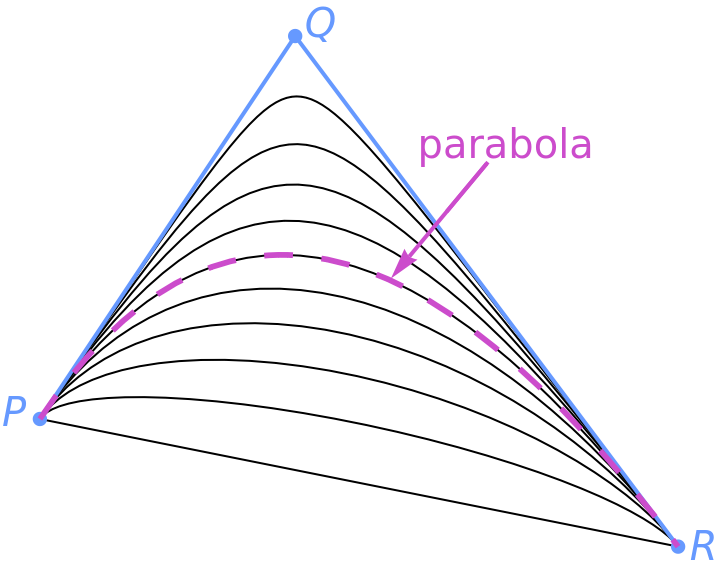
One arc in that family is a portion of a parabola, and all parabolas have eccentricity 1. The arcs that are closer to are portions of hyperbolas; their eccentricities are greater than 1 and grow as they approach . The arcs farther from are portions of ellipses. Their eccentricities fall below 1 as they move away from the parabola, sink to some minimum, and then climb back up to 1 as they approach the base PR of the triangle △PQR (that base here being half of a degenerate ellipse). The minimum at which the eccentricity turns around is 0 just when the triangle △PQR is isosceles, with = , since that’s when an arc of a circle can be inscribed in △PQR.
Q
Q
Q
PQ
QR
All of the arcs in any such family can be drawn as quadratic rational Bézier curves — in Mathematica, as quadratic BSplineCurves with just three control points. With the weights of the two outer control points set to 1, which arc we get is determined by the weight of the middle control point. Setting the middle weight also to 1 gives the parabola, while middle weights less than 1 give ellipses — one of which minimizes the eccentricity.
This notebook, , has interactive diagrams that illustrate two properties of these arcs: the diagonals test and the enveloping ellipse — but with no proofs. The notebook uses the power of Mathematica to give the proofs. In particular, it verifies a formula for the weight that gives the minimum eccentricity, a formula that appeared (without proof) as Equation (3.3) in the paper by Vaughan Pratt, on page 155 of the proceedings of SIGGRAPH-1985. A third notebook, , suggests adding MinEccentricityConic to Mathematica as a new graphics primitive and addresses a problem that arises because the existing primitives JoinedCurve and FilledCurve require certain control points to be omitted.
The tangents at the median crossings
The tangents at the median crossings
This notebook, , has interactive diagrams that illustrate two properties of these arcs: the diagonals test and the enveloping ellipse — but with no proofs. The notebook uses the power of Mathematica to give the proofs. In particular, it verifies a formula for the weight that gives the minimum eccentricity, a formula that appeared (without proof) as Equation (3.3) in the paper by Vaughan Pratt, on page 155 of the proceedings of SIGGRAPH-1985. A third notebook, , suggests adding MinEccentricityConic to Mathematica as a new graphics primitive and addresses a problem that arises because the existing primitives JoinedCurve and FilledCurve require certain control points to be omitted.
The tangents at the median crossings
The tangents at the median crossings
Here is the ellipse from the family above for which the weight of is 1/2, with other things added to the diagram.
Q
In[]:=
With[{p={-2,0},q={0,3},r={3,-1}},{b=(p+r)/2},{m=(b+q/2)/(3/2),n=(b-q/2)/(1/2),c=(b-q/4)/(3/4)},Graphics[{BSplineCurve[{p,q,r},SplineDegree->2,SplineWeights->{1,1/2,1}],Dashing[{0.03}],BSplineCurve[{p,q,r},SplineDegree->2,SplineWeights->{1,-1/2,1}],Dashing[{}],StandardBlue,Text[Style["P",20,Italic],{-2.1,0.25}],Text[Style["Q",20,Italic],{0.25,3.1}],Text[Style["R",20,Italic],{3.15,-0.75}],PointSize[.03],Point[{p,q,r}],Thick,Line[{p,q,r}],StandardGreen,Point[{b,m,n,c}],Text[Style["B",20,Italic],{0.7,-0.25}],Text[Style["M",20,Italic],{0.55,0.92}],Text[Style["N",20,Italic],{1.2,-3.75}],Text[Style["C",20,Italic],{0.9,-1.5}],StandardGray,Line[{2q-b,3b-2q}],StandardBrown,Dashing[{0.03}],Line[{m-3(p-r),m+3(p-r)}],Line[{n-3(p-r),n+3(p-r)}],StandardBlue,Line[{3p-2r,3r-2p}],Dashing[{}]},PlotRange->{{-3,4.5},{-5,3.4}}]]
Out[]=
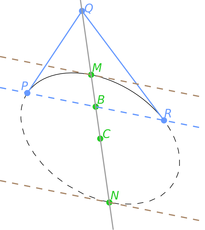
Let be the midpoint of the base of the control triangle. The median of the control triangle is the line , joining that midpoint to the apex .
B=(P+R)/2
PR
BQ
B
Q
Each conic arc in the family crosses the median at the point , that point being the location of the quadratic rational Bézier curve at time . Furthermore, the tangent to the arc at that crossing point is parallel to the base of the control triangle.
BQ
M=(B+sQ)/(1+s)
t=1/2
M
PR
We can complete each conic arc into a full conic by letting vary from 1 up to and then from back to 0. That portion of the conic crosses back over the median line outside of the control triangle at the point , which is the location of the curve at time . The tangent at this crossing point is also parallel to the base .
t
+∞
-∞
BQ
N=(B-sQ)/(1-s)
t=∞
PR
Since the tangents at the median crossings and are parallel, the center of the conic is just the midpoint of the line segment , so we have . Note that always lies on the median line .
M
N
C
MN
C=(B-Q)
2
s
(1-)
2
s
C
BQ
Here is a diagram in which you can drag the three control points around and also set the weight with . When gets all the way to 1, the points and have moved off to infinity, as the ellipse opened out into a parabola.
s
0<=s<=1
s
N
C
If you are using Mathematica to evaluate your own copy of this notebook, then the graphics in interactive diagrams like this one will update continuously as you drag a control point. If you are using a browser to interact with a copy of this notebook in the Wolfram cloud, then the graphics won’t update until you finish your drag, unfortunately.
In[]:=
b[p_,r_]:=(p+r)/2
In[]:=
m[p_,q_,r_,s_]:=(b[p,r]+sq)/(1+s)
In[]:=
n[p_,q_,r_,s_]:=(b[p,r]-sq)/(1-s)
In[]:=
c[p_,q_,r_,s_]:=(b[p,r]-q)(1-)
2
s
2
s
In[]:=
fullConic[{p_,q_,r_},s_]:={BSplineCurve[{p,q,r},SplineDegree->2,SplineWeights->{1,s,1}],Dashing[{0.03}],BSplineCurve[{p,q,r},SplineDegree->2,SplineWeights->{1,-s,1}],Dashing[{}]}
In[]:=
drawTangents[{p_,q_,r_},s_]:={StandardBrown,Dashing[{0.03}],Line[{m[p,q,r,s]-3(p-r),m[p,q,r,s]+3(p-r)}],Line[{n[p,q,r,s]-3(p-r),n[p,q,r,s]+3(p-r)}],StandardBlue,Line[{3p-2r,3r-2p}],Dashing[{}]}
In[]:=
Manipulate[Graphics[{Thickness[0.006],StandardBlue,Line[{p,q,r}],StandardGreen,fullConic[{p,q,r},s],PointSize[0.025],Point[{m[p,q,r,s],n[p,q,r,s]}],StandardGray,Line[{q+10(2q-p-r),q-10(2q-p-r)}],Point[{c[p,q,r,s]}],If[showTangents,drawTangents[{p,q,r},s]]},PlotRange->8,ImageSize->{350,300}],{{p,{-2,0}},Locator},{{q,{0,3}},Locator},{{r,{3,-1}},Locator},{{s,1/2},0,0.99999},(*Lettings=1woulddividebyzero.*){{showTangents,False},{False,True}},LabelStyle->14,SaveDefinitions->savingDefinitions]
The weight that minimizes the eccentricity
The weight that minimizes the eccentricity
There is a surprisingly simple formula for the weight of the apex that produces the conic arc with the minimum eccentricity:
That formula is all that we need to start playing around with min-eccentricity conic arcs, here shown in red:
The diagonals test
The diagonals test
To illustrate that relationship, we need some complicated formulas that compute the aligned bounding box of any inscribed ellipse. Here are those formulas, which aren’t justified in this notebook.
Using those formulas, we can enrich the previous drawing by including the aligned bounding box of the min-eccentricity ellipse, as well as its diagonals.
Here’s a fancier diagram that explores this phenomenon in more detail Along with dragging the three control points, you can here also set the independent weight greenS. That weight determines the green ellipse that is inscribed in the control triangle, with its green aligned bounding box and diagonals. The red arc is the arc of minimum eccentricity, as before, while the blue dashed line is the base of the control triangle.
As greenS increases, the purple phase angle increases from 0, the phase of the base, to the phase of the median, overshoots the latter a bit, and then returns to the phase of the median. The orange phase angle falls to some negative value before returning to 0 and then continuing up to the phase of the median.
Quadrants of ellipses
Quadrants of ellipses
is the square of the hypotenuse of a right triangle, while the denominator is twice the sum of the squares of the two legs. By the Pythagorean Theorem, that quotient is 1/2.
The enveloping ellipse
The enveloping ellipse
Note that the limiting red ellipse is internally tangent to the enveloping green ellipse twice, at points that are antipodal on both ellipses. And the brown tangent lines at those two points are orthogonal to the gray and blue lines, which are at the phase θ.
Drawing a min-eccentricity half ellipse
Drawing a min-eccentricity half ellipse
Here is another diagram with additional lines and curves drawn, to explain why this strategy works: