Arcs of circles that can be Joined
Arcs of circles that can be Joined
Lyle Ramshaw, lyle.ramshaw@gmail.com
I often want to fill a planar region whose boundary includes arcs of circles. But the circular arcs drawn by the primitive Circle can’t be included as segments in a JoinedCurve or FilledCurve. This notebook, , discusses two alternatives.
Specifying the tangent of the arc-to-chord angle
Specifying the tangent of the arc-to-chord angle
It takes five real parameters to specify an arc of a circle. The arcs drawn by the primitive Circle are specified by giving the two coordinates of the circle’s center, its radius, and the arc’s start and stop angles. To specify a circular arc that could be included in a JoinedCurve or FilledCurve, we should instead give the two coordinates of its start and stop points and one additional parameter.
One choice for that fifth parameter is the tangent of the angle that the arc makes at the start point with the chord that joins the start point to the stop point. Setting that tangent to zero gives, as the resulting arc, the chord itself. Setting the tangent to gives the quarter circle that starts anticlockwise of the chord and travels around its circle clockwise, curving to the right to reach its stop point. Setting the tangent to gives the quarter circle that starts clockwise of the chord and travels around its circle anticlockwise, curving to the left to reach its stop point. As the tangent approaches plus or minus infinity, the resulting arc approaches a clockwise or anticlockwise semicircle.
+1
-1
We can implement that primitive using a BSplineCurve with a single rational quadratic segment:
In[]:=
CircularArc[{start_,stop_},tan_]:=Module{chordVec,chordMid,apex},chordVec=stop-start;chordMid=(start+stop)2;apex=chordMid+tan{-chordVec[[2]],chordVec[[1]]}2;BSplineCurve{start,apex,stop},SplineDegree->2,SplineWeights->1,1Sqrt[+1],1
2
tan
By the way, that single rational quadratic segment could be described as a rational quadratic Bézier curve --- but the Mathematica primitive BezierCurve draws only polynomial curves, not rational ones.
Drag the slider below to try out different values for the tangent parameter:
In[]:=
Manipulate[Graphics[{Red,CircularArc[{{-1,0},{1,0}},tan],Blue,PointSize[0.02],Point[{{-1,0},{0,tan},{1,0}}],Line[{{-1,0},{0,tan},{1,0}}],Dashing[{0.03}],Line[{{-1,0},{1,0}}],Dashing[{}],Black,Text[Style["start",14],{-1.18,0.05}],Text[Style["stop",14],{1.15,0.05}],Text[Style["chord",14],{-0.3,0.06}],Text[Style["apex",14],{0.18,tan+0.01}]},PlotRange->{{-1.3,1.3},{-1.5,1.5}}],{{tan,1},-4,4,Appearance->"Labeled",ControlType->VerticalSlider,ControlPlacement->Right},LabelStyle->14,SaveDefinitions->True]
Out[]=

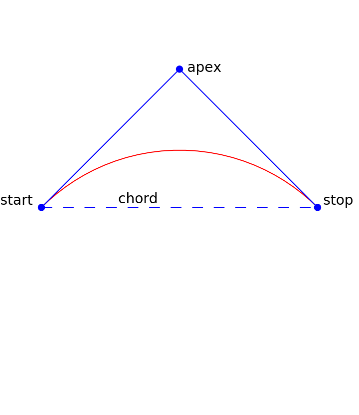
The code above comes close to drawing a semicircle when the tangent parameter is large — perhaps . If we liked, we could test for the tangent being ±∞ and respond by drawing an exact semicircle, drawing it as a Sequence of two quarter circles.
±10000
Arcs of conics that minimize eccentricity
Arcs of conics that minimize eccentricity
We can provide more graphical power to our clients by drawing, not just arcs of circles, but arcs from a six-parameter family: the arcs of conics that minimize their eccentricity.
We give our client independent control over the three points “start”, “apex”, and “stop”, which we now rename , , and (but spell as , , and in Mathematica code). Consider the arcs of conics that begin at , heading toward , and end at , heading away from . Here are some sample arcs from one such family:
P
Q
R
p
q
r
P
Q
R
Q
In[]:=
With[{p={-2,0},q={0,3},r={3,-1}},Graphics[{Table[BSplineCurve[{p,q,r},SplineDegree->2,SplineWeights->{1,s,1}],{s,Table[N[TanDegrees[t]],{t,0,81,9}]}],StandardBlue,Text[Style["P",20,Italic],{-2.2,0.05}],Text[Style["Q",20,Italic],{0.2,3.1}],Text[Style["R",20,Italic],{3.2,-1}],PointSize[.02],Point[{p,q,r}],Thick,Line[{p,q,r}],StandardPurple,Arrowheads[0.044],Arrow[{{1.5,2},{0.75,1.1}}],Thickness[0.008],Dashing[{0.04}],BezierCurve[{p,q,r}],Text[Style["parabola",20],{1.65,2.15}]}]]
Out[]=
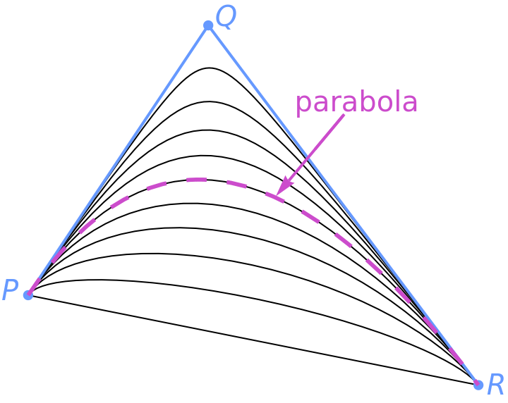
One such arc is the Bézier quadratic polynomial arc, which is an arc of a parabola --- and hence has eccentricity 1. Out closer to , there are arcs of hyperbolas, with eccentricity exceeding 1. Farther from , there are arcs of ellipses. Their eccentricity drops to some minimum and then climbs back up to 1 as they approach the base PR of the control triangle (which here is half of a degenerate ellipse). Somewhere in the middle is the arc that minimizes the eccentricity; and that arc will be circular, with eccentricity 0, just when the control triangle is isosceles, with ==.
Q
Q
△PQR
PQ
QR
All of those conic arcs can be realized exactly as BSplineCurves with one rational quadratic segment simply by varying the weight of the apex , if we leave the weights of and at 1. That varying weight, along with the two coordinates of each of the three control points, is the seventh parameter needed to specify an arc of a conic. We reduce this to six parameters by setting that weight to minimize the eccentricity. The formula for that weight appeared (without proof) as Equation (3.3) in the paper by Vaughan Pratt, on page 155 of the proceedings of SIGGRAPH-1985.
Q
P
R
In[]:=
minimizingWeight[{p_,q_,r_}]:=Sqrt[(p-r).(p-r)/(2((p-q).(p-q)+(q-r).(q-r)))]
In[]:=
MinEccentricityConic[{p_,q_,r_}]:=BSplineCurve[{p,q,r},SplineDegree->2,SplineWeights->{1,minimizingWeight[{p,q,r}],1}]
In[]:=
Manipulate[Graphics[{Blue,Line[{p,q,r}],Red,MinEccentricityConic[{p,q,r}]},PlotRange->8],{{p,{-2,0}},Locator},{{q,{0,3}},Locator},{{r,{3,-1}},Locator},LabelStyle->14,SaveDefinitions->True]
Out[]=
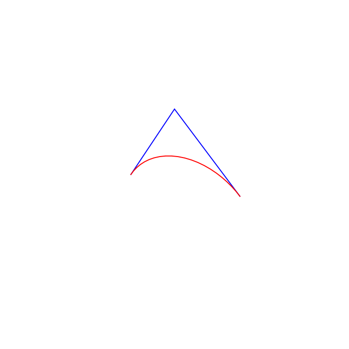
Try dragging the control points around. Note that, when the endpoints and are close together, the red arc of the min-eccentricity conic connecting them stays pretty close to them, even if the apex is a long way away.
P
R
Q
If you are using Mathematica to evaluate your own copy of this notebook, then the graphics in interactive diagrams like this one will update continuously as you drag a control point. If you are using a browser to interact with a copy of this notebook in the Wolfram cloud, then the graphics won’t update until you finish your drag, unfortunately.
The notebook has interactive diagrams that illustrate two properties of these arcs: the diagonals test and the enveloping ellipse — but without proofs. The notebook uses the power of Mathematica to give the proofs. In particular, that latter notebook proves that Pratt’s formula does indeed minimize the eccentricity.
A coding detail: In the degenerate case when , Pratt’s formula divides by zero. The weight doesn’t matter in this case, but it is polite to avoid generating an error message:
P==Q==R
In[]:=
minimizingWeight[{p_,q_,r_}]:=If[p==q==r,1,Sqrt[(p-r).(p-r)/(2((p-q).(p-q)+(q-r).(q-r)))]]
Comparing those two options
Comparing those two options
It’s not clear whether CircularArc or MinEccentricityConic will be more useful in practice. CircularArc is simpler and makes it easy to draw quarter circles. For fractions of a circle other than a quarter, though, computing the proper value for the tangent parameter might be annoying. MinEccentricityConic draws quarter circles with almost equal ease, draws other circular arcs without needing a numerical tangent, does reasonable things when the control triangle is not isosceles, and has intriguing geometric properties to boot. Those advantages may more than repay the hassle of providing a third control point.
One advantage of that third control point is that MinEccentricityConic works fine when its control points are in 3-space, producing an arc that lies in the plane that they span. CircularArc, on the other hand, works only in the plane. Without a third control point, there would be no way to determine which plane in 3-space should contain the circular arc.
The problem of omitted control points
The problem of omitted control points
While CircularArcs and MinEccentricityConics work fine when standing alone, they can’t be included as segments in a JoinedCurve in the way that Lines, BezierCurves, and BSplineCurves can. More precisely, they can’t be so included as any segment other than the first segment of their component. For each adjacent pair of segments in a component, the primitive JoinedCurve requires that the first control point of the latter segment be omitted, filled in by the rendering pipeline with a copy of the last control point of the former segment, thus guaranteeing that the joined curve won’t have a discontinuous jump. But I can’t omit the first control point of either a CircularArc or a MinEccentricityConic --- I need to know that control point to do my calculations.
To address this, I here define a new primitive that behaves just like JoinedCurve, except that no control points are ever omitted. I call this new primitive JoinableCurve --- that is, a joined curve whose segments haven’t yet been joined up. If JoinableCurve is given two adjacent segments that don’t match up, it bridges the gap by inserting an additional line segment. CircularArcs and MinEccentricityConics work fine as segments in a JoinableCurve.
Note that JoinedCurve itself already inserts line segments to bridge some gaps. When the option ClosedCurve is True, the first control point of the first segment of each component should match the last control point of the last segment. JoinedCurve doesn’t guarantee continuity in this case by requiring that one of those two control points be omitted. Instead, it inserts an additional line segment when necessary. JoinableCurve treats all joints in that latter way; so it could be argued that JoinableCurve is actually more consistent than JoinedCurve. JoinableCurve also avoids the confusion of calls to BSplineCurve in which fewer control points than weights are visible, even though the control points and the weights are always in one-to-one correspondence.
The primitive FilledCurve raises the same issues as JoinedCurve, and I resolve them in the same way: by defining a new primitive FillableCurve. (Unless someone can suggest a better name?)
The primitives JoinableCurve and FillableCurve
The primitives JoinableCurve and FillableCurve
Here are implementations of JoinableCurve and FillableCurve that were largely suggested by Mathematica’s large-language model.
An example FillableCurve
An example FillableCurve
Here is a sketch of the BMW logo as a FillableCurve using CircularArcs:
The single component consists of an anticlockwise quarter circle from 12 o’clock to 9 o’clock, then a line segment to 3 o’clock, then a clockwise quarter circle from 3 o’clock to 6 o’clock, and then a line segment back up to 12 o’clock.
Note that both line segments would have been inserted automatically by FillableCurve, had they been omitted from the list of segments. Indeed, any Line segment in a JoinableCurve or FillableCurve that isn’t adjacent to another Line segment could be omitted without affecting the result --- but those omissions are entirely optional.