MinEccentricityConics Analyzed
MinEccentricityConics Analyzed
Lyle Ramshaw, lyle.ramshaw@gmail.com
Introduction
Introduction
Let’s say that an arc of a conic is inscribed in a control triangle △PQR when it starts at , tangent to PQ, and end at R, tangent to QR. Given a control triangle with positive area, there is a one-parameter family of conic arcs that are inscribed in it. One of those arcs has the minimum eccentricity. It’s typically an arc of an ellipse, but it’s an arc of a circle in the special case that the control triangle is isosceles, with = .
P
PQ
QR
In[]:=
With[{p={-2,0},q={0,3},r={3,-1}},Graphics[{Table[BSplineCurve[{p,q,r},SplineDegree->2,SplineWeights->{1,s,1}],{s,Table[N[TanDegrees[t]],{t,0,81,9}]}],StandardBlue,Text[Style["P",20,Italic],{-2.2,0.05}],Text[Style["Q",20,Italic],{0.2,3.1}],Text[Style["R",20,Italic],{3.2,-1}],PointSize[.02],Point[{p,q,r}],Thick,Line[{p,q,r}],StandardPurple,Arrowheads[0.044],Arrow[{{1.5,2},{0.75,1.1}}],Thickness[0.008],Dashing[{0.04}],BezierCurve[{p,q,r}],Text[Style["parabola",20],{1.65,2.15}]}]]
Out[]=
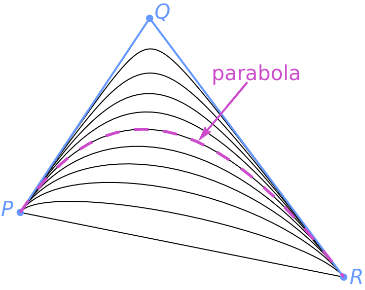
The notebook uses interactive diagrams to illustrate two properties of minimum-eccentricity conics: the diagonals test and the enveloping ellipse — but without proofs. You might want to read that notebook before reading this one. This notebook, , uses the power of Mathematica to give the proofs. In particular, this notebook verifies a formula for the arc with the minimum eccentricity, a formula that appeared (without proof) as Equation (3.3) in the paper by Vaughan Pratt, on page 155 of the proceedings of SIGGRAPH-1985.
There is also a notebook . It suggests adding MinEccentricityConic to Mathematica as a new graphics primitive, and it addresses a problem that arises because the existing primitives JoinedCurve and FilledCurve require certain control points to be omitted.
A warning: Sub-arcs not min-eccentricity
A warning: Sub-arcs not min-eccentricity
Every sub-arc of a circular arc is also a circular arc in its own right — a shorter arc of the same circle; but the analogous property does not hold for min-eccentricity arcs of conics. Among the conic arcs inscribed in some control triangle △PQR, consider the arc that minimizes the eccentricity. Each sub-arc of will be inscribed in a smaller control triangle; but, unless is circular, such a sub-arc typically won’t minimize the eccentricity among the conic arcs inscribed in that smaller control triangle. We will see an example of this below.
The rational quadratic Bézier curve
The rational quadratic Bézier curve
Two coding tidbits: First, in Mathematica code, we’ll write the vertices of the control triangle △PQR as , , and , in lower case. Second, we set a flag about Manipulates:
p
q
r
In[]:=
savingDefinitions=True;
We can draw any conic arc inscribed in the triangle △PQR as a rational quadratic Bézier curve --- in Mathematica, a rational quadratic BSplineCurve with a single segment. To model that curve mathematically, we lift its three control points from the image plane to a 3-space with homogeneous coordinates X, Y, and W, a 3-space in which the image plane is the plane . When doing this lifting, we scale each control point by some positive weight. Multiplying all three weights by any common factor changes nothing; and replacing the weights by for some just gives a different parameterization of the same conic, equivalent to replacing by . So there is a single degree of freedom that affects the shape of the arc, which we can exploit by using the weights for some .
{x,y}
W=1
{a,b,c}
{a,bu,c}
2
u
u
t
t/((1-u)t+u)
{1,s,1}
s
Here is a quadratic polynomial Bézier curve:
In[]:=
polyBezier[{p_,q_,r_},t_]:=p+2(1-t)tq+r
2
(1-t)
2
t
And here is the quadratic rational analog with the weights :
{1,s,1}
In[]:=
ratBezier[{p_,q_,r_},s_,t_]:=polyBezier[{p,sq,r},t]/polyBezier[{1,s,1},t]
In[]:=
ratBezier[{p,q,r},s,t]
Out[]=
p+2qs(1-t)t+r
2
(1-t)
2
t
2
(1-t)
2
t
Setting to 1 gives the polynomial Bézier quadratic, which is an arc of a parabola, with eccentricity 1.
s
In[]:=
ratBezier[{p,q,r},1,t]==polyBezier[{p,q,r},t]//Simplify
Out[]=
True
Raising above 1 gives an arc of a hyperbola, its eccentricity exceeding 1. Setting to some value between 0 and 1 gives an arc of some ellipse, with eccentricity less than 1. Reducing all the way to 0 realizes the line segment from to as half of an ellipse that has collapsed into a doubled line, the eccentricity having climbed back up to 1. The minimum for the eccentricity occurs at some value of between 0 and 1.
s
s
s
P
R
s
The median crossings
The median crossings
The median of the control triangle △PQR is the line connecting the midpoint of the base to the apex . The rational quadratic Bézier curve crosses that median inside the control triangle at when and crosses it again outside that triangle at when .
BQ
B=(P+R)/2
PR
Q
M=(B+sQ)/(1+s)
t=1/2
N=(B-sQ)/(1-s)
t=∞
In[]:=
b[p_,r_]:=(p+r)/2;
In[]:=
m[p_,q_,r_,s_]:=(b[p,r]+sq)/(1+s)
In[]:=
m[p,q,r,s]==ratBezier[{p,q,r},s,1/2]//Simplify
Out[]=
True
In[]:=
n[p_,q_,r_,s_]:=(b[p,r]-sq)/(1-s)
In[]:=
n[p,q,r,s]==Limit[ratBezier[{p,q,r},s,t],t->∞]//Simplify
Out[]=
True
The derivative of the conic with respect to t is given by
In[]:=
derivConic=D[ratBezier[{p,q,r},s,t],t]//FullSimplify
Out[]=
2(-p(s(-1+t)-t)(-1+t)+rt(1+(-1+s)t)+q(s-2st))
2
(1-2(-1+s)(-1+t)t)
The derivatives at and at are both multiples of , so the tangents to the conic as it passes through and are parallel to the base of the control triangle.
t=1/2
t=∞
r-p
M
N
PR
In[]:=
derivConic/.t->1/2//FullSimplify
Out[]=
2(-p+r)
1+s
In[]:=
Series[derivConic,{t,∞,2}]
Out[]=
-p+r
2(-1+s)
2
t
3
O
1
t
So the center of the conic is the midpoint of the segment :
MN
In[]:=
c[p_,q_,r_,s_]:=(b[p,r]-q)(1-)
2
s
2
s
In[]:=
(m[p,q,r,s]+n[p,q,r,s])/2==c[p,q,r,s]//Simplify
Out[]=
True
Finding an implicit equation
Finding an implicit equation
The x and y coordinates of the rational Bezier satisfy
In[]:=
x==polyBezier[{px,sqx,rx},t]/polyBezier[{1,s,1},t]
Out[]=
x+2s(1-t)t+
px+2qxs(1-t)t+rx
2
(1-t)
2
t
2
(1-t)
2
t
In[]:=
y==polyBezier[{py,sqy,ry},t]/polyBezier[{1,s,1},t]
Out[]=
y+2s(1-t)t+
py+2qys(1-t)t+ry
2
(1-t)
2
t
2
(1-t)
2
t
We use a resultant to eliminate the parameter t from those two equations, getting the left-hand side of an implicit equation for the conic of which our arc is a portion:
In[]:=
implicitLHS=Resultant[xpolyBezier[{1,s,1},t]-polyBezier[{px,sqx,rx},t],ypolyBezier[{1,s,1},t]-polyBezier[{py,sqy,ry},t],t]
Out[]=
2
py
2
rx
2
px
2
ry
2
s
2
qy
2
s
2
qx
2
s
2
s
2
py
2
ry
2
s
2
qy
2
s
2
s
2
qy
2
s
2
s
2
s
2
s
2
py
2
x
2
x
2
ry
2
x
2
s
2
x
2
qy
2
s
2
x
2
s
2
x
2
s
2
x
2
rx
2
px
2
qx
2
s
2
s
2
s
2
s
2
s
2
s
2
qx
2
s
2
s
2
s
2
s
2
s
2
s
2
s
2
s
2
px
2
y
2
y
2
rx
2
y
2
s
2
y
2
qx
2
s
2
y
2
s
2
y
2
s
2
y
We rewrite that left-hand side in the form and record its six coefficients:
a+bxy+c+dx+ey+f
2
x
2
y
In[]:=
weightSCoeffs=CoefficientRules[implicitLHS,{x,y}]/.((lhs_->rhs_):>(Replace[lhs,{{2,0}->a,{1,1}->b,{0,2}->c,{1,0}->d,{0,1}->e,{0,0}->f}]->rhs))
Out[]=
{a-2pyry+-4pyqy+4+4pyry-4qyry,b-2pxpy+2pyrx+2pxry-2rxry+4pyqx+4pxqy-8qxqy-4pyrx+4qyrx-4pxry+4qxry,d-2rx+2pxpyry+2pyrxry-2px+4pyqxqy-4px+4pyqyrx-4rx-8pyqxry+4pxqyry+4qxqyry,c-2pxrx+-4pxqx+4+4pxrx-4qxrx,e2pxpyrx-2py-2ry+2pxrxry-4py+4pxqxqy+4pyqxrx-8pxqyrx+4qxqyrx+4pxqxry-4ry,f-2pxpyrxry+-4pyqxqyrx+4pxrx+4pyry-4pxqxqyry}
2
py
2
ry
2
s
2
qy
2
s
2
s
2
s
2
s
2
s
2
s
2
s
2
s
2
s
2
s
2
py
2
ry
2
s
2
qy
2
s
2
s
2
qy
2
s
2
s
2
s
2
s
2
px
2
rx
2
s
2
qx
2
s
2
s
2
s
2
rx
2
px
2
qx
2
s
2
s
2
s
2
s
2
s
2
s
2
qx
2
s
2
py
2
rx
2
px
2
ry
2
s
2
qy
2
s
2
qx
2
s
2
s
Calculating the eccentricity
Calculating the eccentricity
To understand that formula, let’s start with the homogeneous form of the conic’s implicit equation:
For a nondegenerate conic, this discriminant is positive, zero, or negative according as the conic is a hyperbola, a parabola, or an ellipse.
With the implScore in mind, we can present the general formula for the eccentricity of any nondegenerate conic:
Note that the inner radicand is the sum of two squares, so is always nonnegative.
By the way, there is no hope of extending the definition of eccentricity to apply, in a continuous way, to all degenerate conics --- not even just to pairs of intersecting lines, which are perhaps the least degenerate. Consider two lines that intersect at an angle that isn’t a right angle. Shifting the constant term of their implicit equation in one direction gives a nondegenerate hyperbola whose branches lie in the two wider angular sectors, while shifting it in the other direction gives branches that lie in the two narrower sectors. All of the former hyperbolas have a common eccentricity that is different from the common eccentricity of all of the latter. Here is an example:
So we must be content with defining eccentricity only for nondegenerate conics.
We now have a general formula for the eccentricity, but it has a Sign factor; and differentiating such a formula is often challenging. Fortunately, it’s easy to see that the implScore of our implicit equation is always nonnegative:
The behavior of our eccentricity
The behavior of our eccentricity
Minimizing the eccentricity
Minimizing the eccentricity
Solve finds all three critical points, and the nonzero ones are surprisingly and pleasantly simple! We can rewrite the positive solution to show that both the numerator and denominator of its radicand are sums of squares and are hence nonnegative:
To clarify the influence of the geometry of the control triangle, let’s rewrite that solution yet again, generating vectors as differences of the control points and then taking dot products:
So Pratt’s formula is indeed correct. We record that formula for later use:
Try dragging these control points around to see how the resulting arcs behave.
If you are using Mathematica to evaluate your own copy of this notebook, then the graphics in interactive diagrams like this one will update continuously as you drag a control point. If you are using a browser to interact with the copy of this notebook in the Wolfram cloud, then the graphics won’t update until you finish your drag, unfortunately.
Computing the minimum eccentricity
Computing the minimum eccentricity
So the minimum eccentricity is indeed independent of ρ, depending only on θ. Let’s plot how it varies as a function of θ:
Since each hump is left-right symmetric, we get a simpler formula if we focus on just half of one hump.
The diagonals test
The diagonals test
Using those formulas, here’s a routine that draws the aligned bounding box and its diagonals:
To verify this diagonals test, let’s fix an ellipse ℰ and adopt the axial coordinate system in which that ellipse is in standard position, with its center at the origin and its major and minor axes on the x and y axes. The implicit equation of ℰ is its axial coordinates is simply
We can then calculate, with Reduce, when the minimum eccentricity achievable in the control triangle △PQR is the known eccentricity of ℰ:
A subset-of-arc example
A subset-of-arc example
The enveloping ellipse
The enveloping ellipse
We can now check that no point on the min-eccentricity arc lies on or outside of the enveloping ellipse:
The diagram above suggests that this limiting ellipse is internally tangent to the enveloping ellipse at two points. So we want to solve the equations limImpl and envelImpl simultaneously.
So the coordinates of the point of tangency of the solid-red arc are
And that point does indeed lie on both the enveloping conic:
To determine the slope of the tangent lines at the points of internal tangency, we differentiate the implicit equation for the enveloping ellipse — the simpler one:
So the slope of the common tangent line is
If we return to the previous diagram and ask to draw the bounding box of the red ellipse, we aren’t surprised to see that one of its diagonals lies along the median of the control triangle, while the other is parallel to its base. But it’s interesting that, in this limiting situation, the other diagonal of the bounding box actually lies along the base of the control triangle. Indeed, it consistently coincides with the longest diameter of the enveloping ellipse. It follows that, in this limiting situation, the red bounding box is always inscribed in the dotted circle, the smallest circle that contains the enveloping ellipse.