The COVID-19 outbreak, initially in China and now throughout the world, has captured the interest of a large number of organizations and individuals alike. Some effort has been spent to model (or at least visualize) the geographic spread [JHU][JEP]. There have also been some reports of epidemiological models [TG][PYZ][ZCW][JDL][EGE][AA] that have been developed in an effort to estimate parameters that can be used to project the severity of the outbreak, its duration, and the mortality rate.
This report has to main goals. 1) It aims to put some of these modeling efforts into perspective so that conclusions and predictions can be better understood. We will be using compartmental models that allow one to describe the flow of individuals from one health state to another. We will attempt to employ just the right kinds of compartments and connections that are supported by the available data. As the noted statistician G. E. P. Box admonished us, “All models are wrong, but some models are useful.” It is also important know the assumptions on which the models are predicated. 2) It demonstrates the breadth of the Wolfram Language which makes these analyses relatively straight forward, from the retrieval of data from the web, to modeling and data fitting, to exposition and presentation, all in a single interactive document.
It is instructive to first examine two influenza outbreaks that occurred in 1978 in two different boarding schools. The two populations were well defined in terms of size and the assumption of rapid and uniform mixing. These two examples demonstrate that the reported retrospective data can be analyzed satisfactorily by mechanistically different models, and that limitations of the models sometimes preclude the explanation of all the observations.
Next we explore several epidemiological models for the COVID-19 outbreak, and use data from various provinces to estimate model parameters. We primarily want to see how similar or dissimilar the the outbreaks are to each other, point out the short comings, and make some suggestions for improvements.
Compartmental models
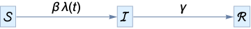
We will be using compartmental models, which have had numerous applications in biology, ecology, chemistry, and medicine. For our purposes, each compartment represents a group of individuals in the same health state, for example susceptible or infectious. The connections between compartments indication the direction and rate of movement from one health state to another. One of the simplest compartmental models for epidemiology has three compartments: susceptible, infectious, and recovered, or SIR. Susceptible individuals come in contact with infectious individuals and become infected. After some period of time, infectious individuals recover, are not longer infectious, and have permanent immunity. The process can be described as a set of transitions
βλ[t]
→
ℐ
infection
ℐ
γ
→
ℛ
recovery
Schematically, the model looks like this
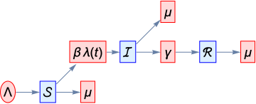
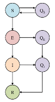
For clarity, we will use a slightly different form of schematic diagram known as a Petri net, which looks like this
There is code in the Initialization section at the end of the notebook for generating these graphs.
This transmission model describes the rate of change of each of the compartments, which can be modeled mathematically as a system of ordinary differential equations (ODEs).
′
[t]-β[t]λ[t]
′
ℐ
[t]-γℐ[t]+β[t]λ[t]
′
ℛ
[t]γℐ[t]
λ[t]ℐ[t]
The number of infectious individuals in the population
ℐ[t]
is the prevalence of the disease. The number of individuals that become infected per unit time is called the incidence.
Many epidemiologic models include population demographics, that is, birth and natural death. For comparison, this is the SIR model with demographics
Because the duration of the influenza and COVID-19 outbreaks that are discussed here are so short (weeks or months), we can make the assumption that births and natural deaths can be ignored.
These compartmental models and their ODE representation were first developed by Kermack and McKendrick [KM] almost 100 years ago. One of the assumptions is that the population of individuals is well mixed, that is, every individual has equal likelihood to come into contact with every other individual. This assumption rarely holds in practice, but useful results can be obtained nonetheless. Other assumptions to keep in mind are that all individuals in each class are identical, and that recovery confers life-long perfect immunity.
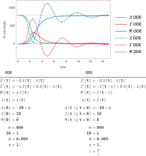
While delay differential equations (DDE) are often used in population models for ecology, and many other areas as well, they can lead to unphysical artefacts. For example, shown below is the SIR model solution (solid curves) and the solution for the corresponding DDE model (dashed curves). While the total population size (
[t][t]+ℐ[t]+ℛ[t]
) is constant, the infected compartment in the DDE model (dashed red) has several excursions below 0 and the recovered compartment (dashed blue) has corresponding excursions above . Adding a scaling factor to those terms in the DDEs will only minimize and not eliminate the issue. The oscillations are also of concern.
While DDE models have been used for epidemiological models [AV], they must be used with care.
Parameter optimization
All of the parameters in these model need to remain in the range
(0,∞)
or
(0,1)
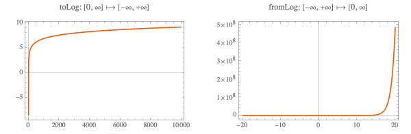
, so constraints should be used. Wolfram Language has many efficient functions for optimization with constraints, and for many systems they work well. From many years of experience with these kinds of models (epidemiologic, pharmacokinetic, and viral dynamics), a simpler passive constraint method (transformation) with unconstrained optimization works better.
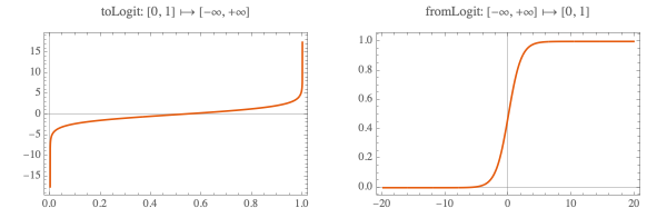
Values for parameters that should fall between 0 and ∞ are log-transformed and the parameters in the ODEs are back-transformed with
Exp
. Similarly, for parameters whose values should be between 0 and 1 we use the logit transformation and its inverse. To facilitate coding, the functions
There are two textbook examples of influenza outbreaks in boarding schools. They are retrospective reports because the studies were unplanned, however, from a modeling perspective they present several advantages:
◼
The populations were closed (no migration in or out)
◼
There were no births or deaths, so models without demographics can be used
◼
The populations were well mixed as the students were attending classes together
◼
There is a daily record of the number of students with influenza
The data
Outbreak 1
Dataset
◼
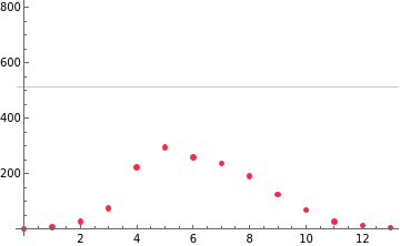
From a textbook problem, Martcheva. pp. 126-139 [MM][A]
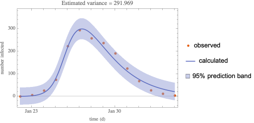
…, in January-February 1978, an epidemic of influenza occurred in a boarding school in the north of England. The boarding school housed a total of 763 boys, who were at risk during the epidemic. On January 22, three boys were sick.
512 boys (67%) spent between three and seven days away from class, …
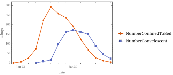
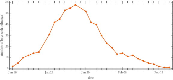
From another textbook problem, Martcheva, pp. 144-145 [MM][HJR]
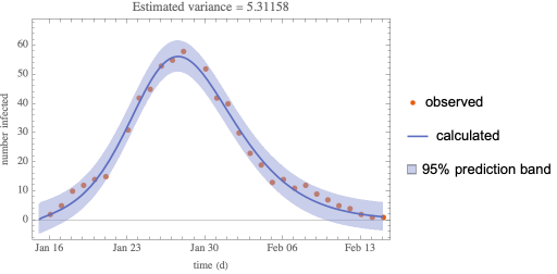
The West Country English Boarding School housed 578 boys. An epidemic of influenza began on 15 January 1978.
One hundred and sixty-six boys (29 per cent) were treated in the sick bays by bed rest and aspirin. Certainly this is not the total number with influenza, as the older boys had their own rooms in which some remained, treating themselves and avoiding detection and supervision as a result of the dislocated curriculum.
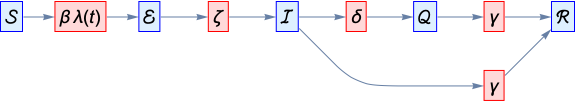
Since the data report the “number of boys confined to bed”, they are actually quarantined or isolated and not freely circulating among the student body
◼
SEIQR: SEIR model with quarantined compartment
◼
No birth or natural mortality due to short time span of coverage of model
We will examine datasets assuming the first infections occurred on 20 Dec 2019, and 30 Dec 2019 (when the first reported infections)
◼
The initial number of infected individuals
I0
is
10
; Du et al. estimated the number to be 7.78 in Wuhan [DWC]
◼
Even though the severity of the infection and risk of death have been reported to be age- and gender-dependent, the available data for modeling does not have sufficient detail to support stratification by age and gender
◼
Under reporting of cases is a serious concern, primarily due to the infection being asymptomatic in many individuals, especially children [CXL]; we will assume that all cases are reported
◼
This work was carried out over a number of days, with the available WDR data keeping pace. However to assure a consistent analysis and interpretation of results we’ll work with data for the period 21 Jan 2020 to 26 Feb 2020.
◼
More recent data can be used to test the models.
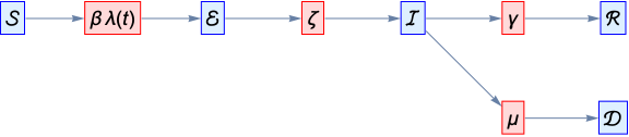
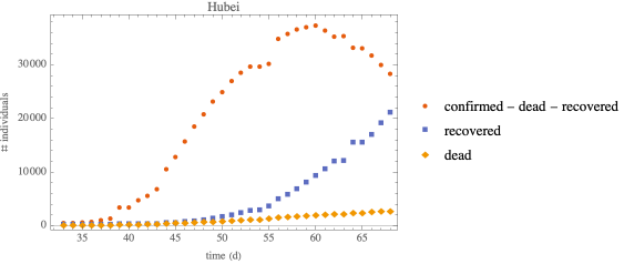
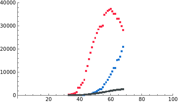
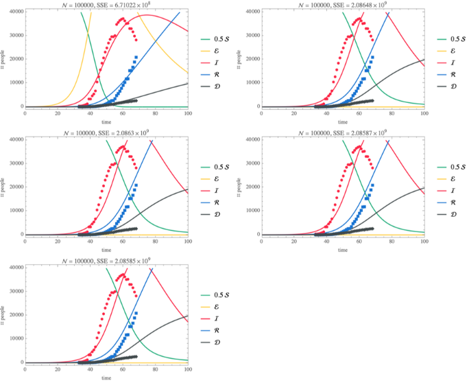
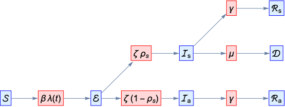
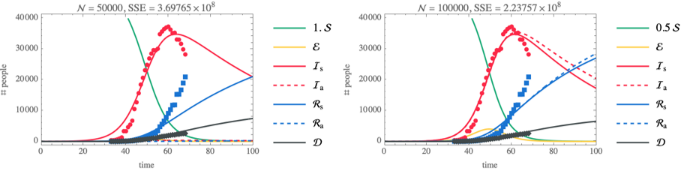
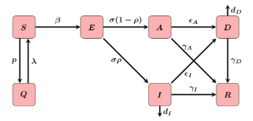
Hubei outbreak—SEIRD
SEIRD Model with standard incidence
◼
SEIRD: SEIR model with dead compartment
◼
An effective population size
with standard incidence will be used
◼
This assumes that individuals in the population cannot come in contact with all other individuals in the population; this is in contrast to models for influenza and SARS [MM]
◼
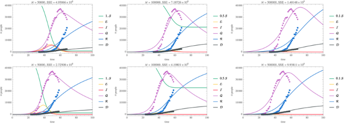
may be adjusted for individual locations; initially we'll use
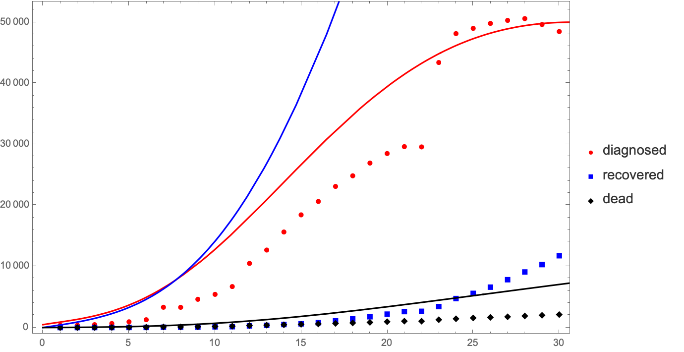
remove the jump in confirmed cases in Hubei that occurred when the testing method changed, which at the time seemed like a reasonable data preprocessing step. Unfortunately, for the data after about 15 March 2020 this practice leads to an artefact that gives negative values.
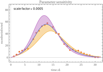
increasing the population size makes ℐ peak broader
◼
shifting t0 to a later date (closer to the data) does not have a noticeable effect
◼
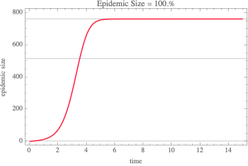
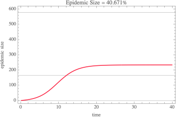
in all cases, the susceptible compartment goes to 0 and the epidemic size is 100% of the population
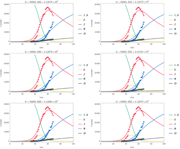
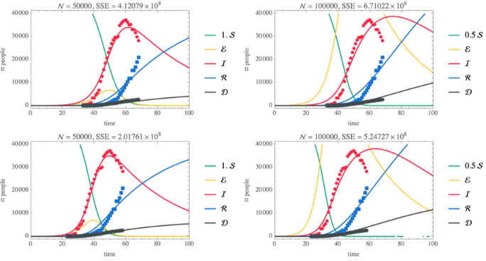
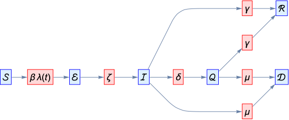
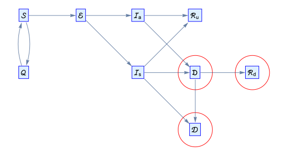
Hubei outbreak—SEIQRD
SEIQRD Model with standard incidence
◼
SEIQRD: SEIQR model with dead compartment
◼
Quarantined individuals
[t]
do not contribute to the force of infection
◼
The duration of circulation of infected individuals is constant even though we know it was initially infinitely long and later became very short as isolation and quarantine measures were instituted, however no detailed information about when changes occurred is available
◼
The duration of infection and the mortality rate for circulating and quarantined infectious individuals is the same
[ZCW] Y. Zhou, Z. Chen, X. Wu, Z. Tian, L. Cheng, L. Ye “The Outbreak Evaluation of COVID-19 in Wuhan District of China”, https://arxiv.org/pdf/2002.09640.pdf
[JDL] J. Jia, J. Ding, S. Liu, G. Liao, J. Li, B. Duan, G. Wang, R. Zhang “Modeling the Control of COVID-19: Impact of Policy Interventions and Meteorological Factors”, https://arxiv.org/pdf/2003.02985.pdf
[AV] J. Arino, P. van den Driessche “Time delays in Epidemic Models; Modeling and Numerical Considerations” in “Delay Differential Equations and Applications”, O. Arino (ed.) Springer, 2006.
[BCR] M. Biggerstaff, S. Cauchemez, C. Reed, M. Gambhir, L. Finelli “Estimates of the reproduction number for seasonal, pandemic, and zoonotic influenza: a systematic review of the literature” BMC Infectious Diseases, 14, 480 (2014), http://www.biomedcentral.com/1471-2334/14/480
[MM] M. Martcheva “An introduction to mathematical epidemiology” Springer, 2015.
[HJR] H. J. Rose “The use of amantadine and influenza vaccine in a type A influenza epidemic in a boarding school”, Journal of Royal College of General Practitioners, 30, 619-621 (1980). PubMedCentral
[FT] Z. Feng, H. R. Thieme “Recurrent Outbreaks of Childhood Diseases Revisited: The Impact of Isolation”, Math. Biosciences, 128, 93-130 (1995). https://doi.org/10.1016/0025-5564(94)00069-C
[DWC] Z. Du, L. Wang, S. Cauchemex, X. Xu, X. Wang, B. J. Cowling, L. A. Meyers “Risk for Transportation of 2019 Novel Coronavirus (COVID-19) from Wuhan to Cities in China”, https://doi.org/10.1101/2020.01.28.20019299
[CXL] J. Cai, J. Xu, D. Lin, Z. Yang, L. Xu, Z, Qu, Y. Zhang, H. Zhang, R. Jia, P. Liu, X. Wang, Y. Ge, A. Xia, H. Tian, H. Chang, C. Wang, J. Li, J. Wang, M. Zheng “A Case Series of children with 2019 novel coronavirus infection: clinical and epidemiological features”, Clinical Infectious Diseases, https://doi.org/10.1093/cid/ciaa198
[CWB] B. J. Coburn, B. G. Wagner, S. Blower “Modeling influenza epidemics and pandemics: insights into the future of swine flu (H1N1)”, BMC Medicine, 7, (2009), http://www.biomedcentral.com/1741-7015/7/30