Epidemiological Models for Influenza and COVID-19
Epidemiological Models for Influenza and COVID-19
Robert B. Nachbar
Original post: 11-Mar-2020
Revised: 15-Mar-2020
Revised: 9-Apr-2020
◼
The package should be in the same directory as the notebooks, and is automatically loaded as part of the initialization.
Table of Contents
Table of Contents
◼
Use the subsection cells to navigate to the other notebooks
COVID-19
COVID-19
◼
Models
◼
SEIsaRD Model with standard incidence
◼
Hubei outbreak—SEIsaRD
◼
Outbreak start 20 Dec 2019
◼
Fitting data
◼
Manual fit
◼
Optimization—
100000
◼
Optimization—
50000
◼
Comparisons
References
References
Initialization
Initialization
COVID-19
Models
Models
SEIsaRD Model
SEIsaRD Model
◼
These are the ODEs
forceOfInfectionSEIsaRD=λ[t_][t]+[t];{varsSEIsaRD,odesSEIsaRD}=Values@KineticCompartmentalModelℰ,ℰ,ℰ,,,,t{1,-1};Column[odesSEIsaRD]
ℐ
"s"
ℐ
"a"
-[t]
βλ[t]
→
ζρ
→
ℐ
"s"
ζ(1-ρ)
→
ℐ
"a"
ℐ
"s"
γ
→
ℛ
"s"
ℐ
"a"
γ
→
ℛ
"a"
ℐ
"s"
μ
→
Out[]=
′ ℐ s |
′ ℰ |
′ |
′ ℐ a ℐ a |
′ ℐ s ℐ s ℐ s |
′ ℛ a ℐ a |
′ ℛ s ℐ s |
{susceptibleSEIsaRD,exposedSEIsaRD,infectedSymptomaticSEIsaRD,infectedAsymptomaticSEIsaRD,recoveredSymptomaticSEIsaRD,recoveredAsymptomaticSEIsaRD,deadSEIsaRD}={,ℰ,,,,,}/.ParametricNDSolve[Join[odesSEIsaRD/.forceOfInfectionSEIsaRD,{[0]-I0,ℰ[0]0,[0]ρI0,[0](1-ρ)I0,[0]0,[0]0,[0]0}],varsSEIsaRD,{t,0,500},{,I0,β,ζ,ρ,γ,μ}];
ℐ
"s"
ℐ
"a"
ℛ
"s"
ℛ
"a"
ℐ
"s"
ℐ
"a"
ℛ
"s"
ℛ
"a"
Hubei outbreak—SEIsaRD
Hubei outbreak—SEIsaRD
Outbreak start 20 Dec 2019
Outbreak start 20 Dec 2019
Fitting data
Fitting data
In[]:=
t0=DateObject["20 Dec 2019"]
Out[]=
In[]:=
fitData1=fitData=fitDataWDR,t0,"makeCorrectionForHubei"True,"dateRange"{All,"26 Feb 2020"};Dimensions/@%
Out[]=
{{36,2},{36,2},{36,2}}
In[]:=
ListPlot[fitData,PlotLabel"Hubei",FrameLabel{"time (d)","# individuals"},PlotLegends{"confirmed"-("recovered"+"dead"),"recovered","dead"}]
Out[]=

Manual fit
Manual fit
Out[]=


Optimization—100000
Optimization—
100000
Optimization—50000
Optimization—
50000
Comparisons
Comparisons
In[]:=
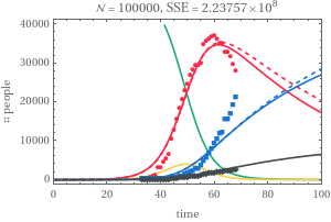
{2.237574248580851`*^8,{logBeta-1.431643518034431`,logZeta0.17799734382500643`,logitRho0.037767138874603576`,logGamma-4.042140864793616`,logMu-5.461954934030664`}}//Append[MapThread[Compose,{{fromLog,fromLog,fromLogit,fromLog,fromLog},Values@Last@#}],First@#]&
Out[]=
{0.238916,1.19482,0.509441,0.0175598,0.00424525,2.23757×}
8
10
Out[]//TableForm=
startDate | populationSize | β | ζ | ρ | γ | μ | SSE |
20 Dec 2019 | 50000 | 0.201151 | 2.68809 | 0.990566 | 0.0128232 | 0.00454096 | 3.69765× 8 10 |
20 Dec 2019 | 100000 | 0.238916 | 1.19482 | 0.509441 | 0.0175598 | 0.00424525 | 2.23757× 8 10 |
In[]:=
MapThread[plotFitSEIsaRD[#,Insert[#2,10,2],ImageSize300]&,{{fitData1,fitData1(*,fitData2,fitData2*)},Most/@Rest/@bestFits}]//Partition[#,2]&//GridcloseCellGroup[]
Out[]=

◼
Increasing the population size increases the recovery rate
◼
In all cases, the susceptible compartment goes to 0 and the epidemic size is 100% of the population
References
[JHU] “Mapping 2019-nCoV”, https://systems.jhu.edu/research/public-health/ncov/
[TG] T. Götz, “First attempts to model the dynamics of the coronavirus outbreak 2020”, https://arxiv.org/pdf/2002.03821.pdf
[PYZ] L. Peng, W. Yang, D. Zhang, C. Zhuge, L. Hong “Epidemic analysis of COVID-19 in China by dynamical modeling”, https://www.medrxiv.org/content/10.1101/2020.02.16.20023465v1
[ZCW] Y. Zhou, Z. Chen, X. Wu, Z. Tian, L. Cheng, L. Ye “The Outbreak Evaluation of COVID-19 in Wuhan District of China”, https://arxiv.org/pdf/2002.09640.pdf
[JDL] J. Jia, J. Ding, S. Liu, G. Liao, J. Li, B. Duan, G. Wang, R. Zhang “Modeling the Control of COVID-19: Impact of
Policy Interventions and Meteorological Factors”, https://arxiv.org/pdf/2003.02985.pdf
Policy Interventions and Meteorological Factors”, https://arxiv.org/pdf/2003.02985.pdf
[EGE] E. G. M E. “An SEIR like model that fits the coronavirus infection data”, https://community.wolfram.com/groups/-/m/t/1888335
[AA] A. Antonov “Basic experiments workflow for simple epidemiological models”, https://community.wolfram.com/groups/-/m/t/1895686
[AV] J. Arino, P. van den Driessche “Time delays in Epidemic Models; Modeling and Numerical Considerations” in “Delay Differential Equations and Applications”, O. Arino (ed.) Springer, 2006.
[FB] F. Brauer “Reproduction numbers and final size relations”, https://www.fields.utoronto.ca/programs/scientific/10-11/drugresistance/emergence/fred1.pdf
[BCR] M. Biggerstaff, S. Cauchemez, C. Reed, M. Gambhir, L. Finelli “Estimates of the reproduction number for seasonal, pandemic, and zoonotic influenza: a systematic review of the literature” BMC Infectious Diseases, 14, 480 (2014), http://www.biomedcentral.com/1471-2334/14/480
[MM] M. Martcheva “An introduction to mathematical epidemiology” Springer, 2015.
[A] Anonymous, Anonymous, Brit. Med. J., 1978, https://www.ncbi.nlm.nih.gov/pmc/articles/PMC1603269/pdf/brmedj00115-0064.pdf
[HJR] H. J. Rose “The use of amantadine and influenza vaccine in a type A influenza epidemic in a boarding school”, Journal of Royal College of General Practitioners, 30, 619-621 (1980). PubMedCentral
[FT] Z. Feng, H. R. Thieme “Recurrent Outbreaks of Childhood Diseases Revisited: The Impact of Isolation”, Math. Biosciences, 128, 93-130 (1995). https://doi.org/10.1016/0025-5564(94)00069-C
[BK] S. Boseley, L. Kuo “Huge rise in coronavirus cases casts doubt over scale of epidemic”, The Guardian, 13 Feb 2020, https://www.theguardian.com/world/2020/feb/13/huge-rise-coronavirus-cases-raises-doubts-scale-epidemic-china
[DWC] Z. Du, L. Wang, S. Cauchemex, X. Xu, X. Wang, B. J. Cowling, L. A. Meyers “Risk for Transportation of 2019 Novel Coronavirus (COVID-19) from Wuhan to Cities in China”, https://doi.org/10.1101/2020.01.28.20019299
[CXL] J. Cai, J. Xu, D. Lin, Z. Yang, L. Xu, Z, Qu, Y. Zhang, H. Zhang, R. Jia, P. Liu, X. Wang, Y. Ge, A. Xia, H. Tian, H. Chang, C. Wang, J. Li, J. Wang, M. Zheng “A Case Series of children with 2019 novel coronavirus infection: clinical and epidemiological features”, Clinical Infectious Diseases, https://doi.org/10.1093/cid/ciaa198
[CWB] B. J. Coburn, B. G. Wagner, S. Blower “Modeling influenza epidemics and pandemics: insights into the future of swine flu (H1N1)”, BMC Medicine, 7, (2009), http://www.biomedcentral.com/1741-7015/7/30
Initialization
◼
the package can be downloaded from https://www.wolframcloud.com/obj/rnachbar/Published/CompartmentalModeling.wl
General
General
Fitting data
Fitting data
Fitting error
Fitting error
SEIsaRD
SEIsaRD