In[]:=
Fri 6 Jun 2025 16:07:14
Wolfram Three Domains notability.
Formulas for mapping between three domains.
Formulas for mapping between three domains.
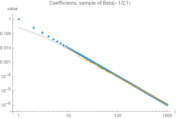
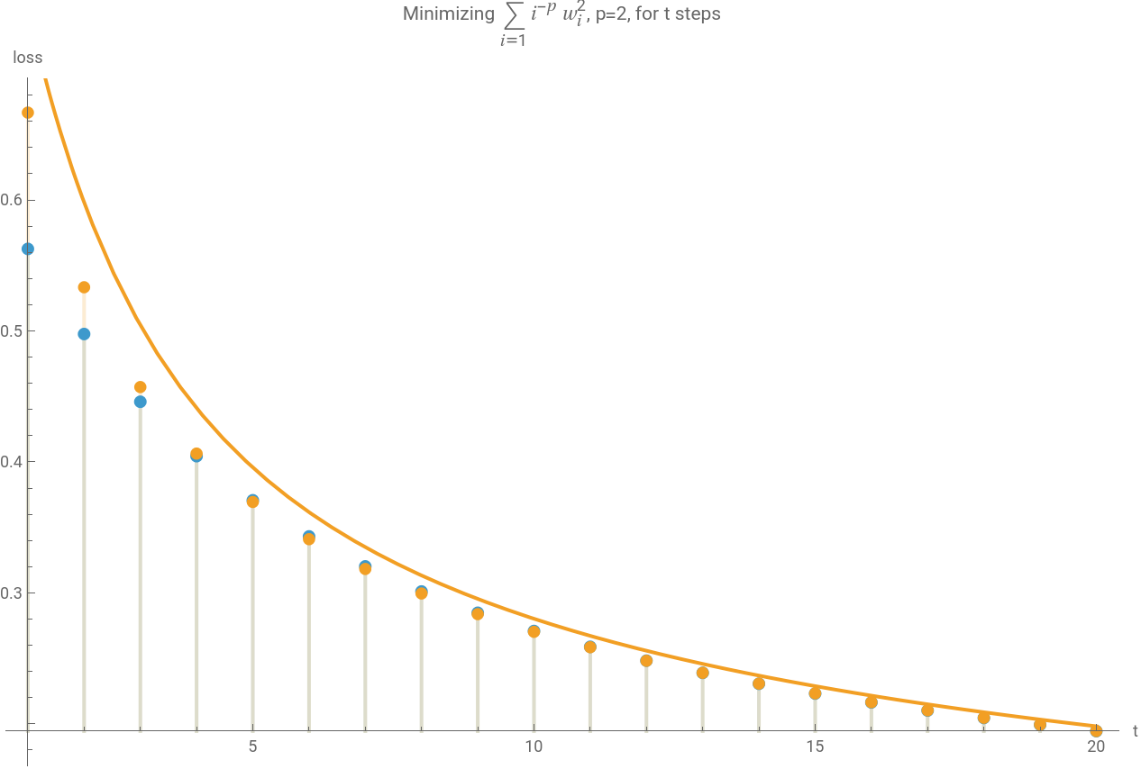
Suppose we have a quadratic with coefficients 1, 1/4, 1/9, 1/16, ...., and we minimize it using gradient descent with learning rate 1. How does the loss behave over time?
We can unlock analytic tools by studying a closely related quadratic with random coefficients.
1. Random Variable (expectations)
2. Density (integral transforms)
3. Sequence of moments (generating functions)
Related:
https://www.wolframcloud.com/obj/yaroslavvb/newton/wolfram-integrals-post.nb
https://www.wolframcloud.com/obj/yaroslavvb/nn-linear/forum-erfc-formula.nb
root: linear-estimation-scratch-2025
chris-desa-scratch.nb
chris-desa: Mapping between three domains for Beta(1/2,1)
1/
2
n
We can unlock analytic tools by studying a closely related quadratic with random coefficients.
1. Random Variable (expectations)
2. Density (integral transforms)
3. Sequence of moments (generating functions)
Related:
https://www.wolframcloud.com/obj/yaroslavvb/newton/wolfram-integrals-post.nb
https://www.wolframcloud.com/obj/yaroslavvb/nn-linear/forum-erfc-formula.nb
root: linear-estimation-scratch-2025
chris-desa-scratch.nb
chris-desa: Mapping between three domains for Beta(1/2,1)
Random quadratic realization
Random quadratic realization
In[]:=
Table[1,{i,1,20}]
2
i
Out[]=
1,,,,,,,,,,,,,,,,,,,
1
4
1
9
1
16
1
25
1
36
1
49
1
64
1
81
1
100
1
121
1
144
1
169
1
196
1
225
1
256
1
289
1
324
1
361
1
400
In[]:=
SeedRandom[1];Needs["MaTeX`"];pretty[expr_]:=MaTeX[expr];SetAttributes[pretty,HoldAll];numCoefs=1000;z=Integrate,x,,1;(*thiscorrespondstotruncatedBetaDistribution[-1/2,1]*)dist=ProbabilityDistribution,x,,1;randomCoefs=Reverse@Sort@RandomVariate[dist,numCoefs];randomCoefs=randomCoefs/First@randomCoefs;myCoefs=Table[,{i,1,numCoefs}];dec[list_]:=With[{n=Length@list},{Range[n],list}];sf={"Log","Log"};coefPlot=ListPlot{dec@myCoefs,dec@randomCoefs},ScalingFunctions->sf,PlotLegends->pretty@,"sorted sample",PlotStyle->{PointSize[Medium],Automatic};expectedPlot=Plot[InverseSurvivalFunction[dist,x/numCoefs],{x,0,numCoefs},ScalingFunctions->{"Log","Log"},PlotStyle->{Directive[Gray,Thickness[.01],Opacity[.2]]},PlotLegends->{"Inverse Survival Function"}];SF=StringForm;Show[coefPlot,expectedPlot,AxesLabel->{"i","value"},PlotLabel->SF["Coefficients, sample of Beta(-1/2,1)"]]
-3/2
x
1
2
numCoefs
1
z
-3/2
x
1
2
numCoefs
-2
i
1
2
i
Out[]=


Check loss (from wolfram-integrals-post.nb *)
In[]:=
dist=BetaDistribution[1/2,1];truthContinuous=Simplify[MomentGeneratingFunction[dist,t]/.t->-t]lossTruePrecision=20;lossTrue[t0_]:=With[{t=SetPrecision[t0,lossTruePrecision],h=},nsumMethod={"EulerMaclaurin",Method{"NIntegrate","MaxRecursion"14,Method"DoubleExponential"}};NSum[h,{i,0,∞},WorkingPrecision->lossTruePrecision-1,MethodnsumMethod]];maxT=20;momentExpr=;momentExpr=;actualPlot=DiscretePlot[{lossTrue[t],momentExpr},{t,1,maxT},PlotLegends->{"true loss",pretty@momentExpr},PlotStyle->{PointSize[Large],Automatic}];SF=StringForm;ShowactualPlot,Plot[{None,truthContinuous},{t,1,maxT},PlotLegends->{pretty@truthContinuous}],PlotLabel->SF"Minimizing , p=``, for t steps",2,AxesLabel->{"t","loss"}
-2
(1+i)
t
(1-h)
t
4
2
(t!)
(1+2t)!
(2t)!!
(1+2t)!!
Out[]=
π
Erf[t
]2
t
Out[]=


Using difference equation vs differential equation
Using difference equation vs differential equation
Difference equation
Difference equation
In[]:=
expr1=Moment[TransformedDistribution[1-,xUniformDistribution[]],n];expr2=Beta1+n,;Column[{expr1==expr2,Table[Simplify[expr1==expr2],{n,1,3}]}]
2
x
1
2
1
2
Out[]=
π Gamma[1+n]2Gamma 3 2 1 2 1 2 |
{True,True,True} |
In[]:=
expr1=RSolveValuea[n]==1-a[n-1],a[0]==1,a[n],nexpr2=Beta1+n,;Column[{expr1==expr2,Table[Simplify[expr1==expr2],{n,1,3}]}]
1
2n+1
1
2
1
2
Out[]=
Pochhammer[1,n]
Pochhammer,n
3
2
Out[]=
Pochhammer[1,n] Pochhammer 3 2 1 2 1 2 |
{True,True,True} |
Differential equation
Differential equation
In[]:=
ClearAll["Global`*"];case1=-1/(2*t);DSolveValuef'[t]==-f[t],f[1]==,f[t],t
1
2t
Pi
2
Out[]=
π
2
t
In[]:=
sol=MomentGeneratingFunction[BetaDistribution[1/2,1],t]/.t->-tAsymptotic[sol,t->∞]
Out[]=
π
Erfi[-t
]2
-t
Unit tests
Unit tests
Density column
Density column
Expectation column
Expectation column
Moment column
Moment column
Beta(1/2,1) Stieltjes and OGF
Beta(1/2,1) Stieltjes and OGF
Uniform Distribution
Uniform Distribution