In[]:=
Wed 17 May 2023 18:55:27
Deriving Erfc formula
Deriving Erfc formula
In[]:=
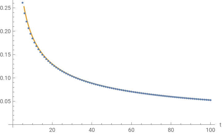
formula=Erfc;formula=1-Erf;getTrueLosses[p_,d_,z_,maxSteps_]:=Module[{},discretize[expr_]:=Table[N@expr,{i,0,d-1}];h$=discretize[/z];steps=Table[t,{t,0,maxSteps}];traj=NestList[#-#*h$&,discretize[1],maxSteps];{steps,h$.&/@traj}];Block[{p=2,d=100,a=-2,maxSteps=100},trueLosses=Rest[Last/@getTrueLosses[p,d,1,maxSteps]];predictedLosses=Table[formula,{t,1,maxSteps}];];ListPlot[{trueLosses,predictedLosses},Joined->{False,True},PlotLegends->{"f(t)",formula},AxesLabel->{"t"}]
2
t
d
π
2
2
t
2
t
d
π
2
2
t
-p
(1+i)
2
#
Out[]=


In[]:=
A=DiagonalMatrix[h$];ii=IdentityMatrix[Length@h$];h$.MatrixPower[ii-A,200,discretize[1]]==Last@trueLosses
Out[]=
True
In[]:=
Tr[A.MatrixPower[ii-A,200]]==Last@trueLosses
Out[]=
True
Obtaining candidate
Obtaining candidate
In[]:=
Clear["Global`*"];baseAssumptions=d>1,1<p<=2,a<0,0<=b<=1,!=1,<1,>0,Log-≠0,Log-!=0;sAssumptions={s>0};(*Trickfromhttps://mathematica.stackexchange.com/questions/284437/inverselaplacetransform-involving-an-arctan*)hackedLaplaceAtan[expr_]:=Module[{expr2,ilap},expr2=expr/.ArcTan[e_]->ArcTan[A*e];ilap=InverseLaplaceTransform[D[expr2,A]//Factor,s,t];Assuming[{t>0},Integrate[ilap,{A,0,1}]]];z=1;(*Changebetweenindexingdomainanddensitydomain*)iDomain[expr_]:=MemberQ[Reduce`FreeVariables[expr],i];yDomain[expr_]:=MemberQ[Reduce`FreeVariables[expr],y];varchange[expr_]:=IfiDomain[expr],expr/.i->-1,Assert[yDomain[expr]];expr/.y->z;h=varchange@y;(*h=/z;*)pdf=;toI[expr_]:=If[iDomain[expr],expr,varchange@expr];toY[expr_]:=If[yDomain[expr],expr,varchange@expr];laplaceDomain[expr_]:=MemberQ[Reduce`FreeVariables[expr],s];timeDomain[expr_]:=MemberQ[Reduce`FreeVariables[expr],t];lap[expr_]:=Block[{$Assumptions=baseAssumptions},If[laplaceDomain[expr],InverseLaplaceTransform[expr,s,t],LaplaceTransform[expr,t,s]]]Ei[expr_]:=Block[{i},Inactive[Integrate][toI[expr],{i,0,d-1}]];Ey[expr_]:=Block[{y},Inactive[Integrate][pdftoY[expr],{y,,1}]];Ehi[expr_]:=Block[{i},Inactive[Integrate][htoI[expr],{i,0,d-1}]];Ehy[expr_]:=Block[{y},Inactive[Integrate][pdfytoY[expr],{y,,1}]];f0=1;z=1;F=;Activate[Ehi@F/.{p->2,a->-2}]//Apart//Expand
p
d
-p
d
p
d
1
a
p
d
a
-1
p
(yz)
-p
(i+1)
-p
(i+1)
1
p
-1/p
z
-(1+1/p)
y
-p
d
-p
d
f0
s-ah
Out[]=
-+
ArcTan
s
2
2
s
ArcTan
d
s
2
2
s
In[]:=
Activate[Ehy@F/.{p->2,a->-2}]//Apart//Expand
Out[]=
-+
ArcTan
s
2
2
s
ArcTan
d
s
2
2
s
In[]:=
hackedLaplaceAtan-+//Apart//Expand
ArcTan
s
2
2
s
ArcTan
d
s
2
2
s
Out[]=
-Erfc[+Erfc
π
2
2
t
]2
t
π
2
2
t
d
2
t
In[]:=
term1=Erfc;term2=-Erfc[;Block{d=100},LogPlotterm1+term2,-,{t,1,100},PlotLabel->"Can we drop second term? (yes)",PlotLegends->{"loss","relative size of second term"},AxesLabel->{"t"}
π
2
2
t
d
2
t
π
2
2
t
]2
t
term2
term1+term2
Asymptotic behavior
Asymptotic behavior
Infinite t asymptotics
Infinite t asymptotics
Infinite d asymptotics
Infinite d asymptotics
Asymptotic Plots
Asymptotic Plots
From mean-field-equation: Exhaustive Solutions