In[]:=
Sat 12 Oct 2024 17:45:58
There’s been a recent interest in optimization community in characterizing the behavior of gradient descent on simple quadratics, for instance, recent work by Francis Bach:- https://francisbach.com/scaling-laws-of-optimization/We are interested in minimizing a quadratic function Hw w.r.t. to w by starting with random point and performing gradient descentWithout loss of generality (see Footnote 1), loss after t steps is described by the following sumBelow I give the tools we can use to better understand behavior of this kind of sum.
′
w
w
0
f(t)
∑
i1
h
i
2t
(1-)
h
i
Footnote 1: Without loss of generality: gradient descent becomes independent of random starting point because of concentration (see this), worst analysis is overly pessimistic in high dimensions (see this and this), gradient descent is invariant to unitary transformation and shift (see this). We fix step size to 1/L where L is the Lipschitz because that’s the largest step size for which algebra is easy. It’s also within a factor of 2 of “largest step size possible”, therefore our step-time-complexity has efficiency at least 0.5 of step-time-complexity of gradient descent with “constant optimally tuned learning rate”.
Pre-requisites
Tool 1: continuous time and continuous state
Tool 1: continuous time and continuous state
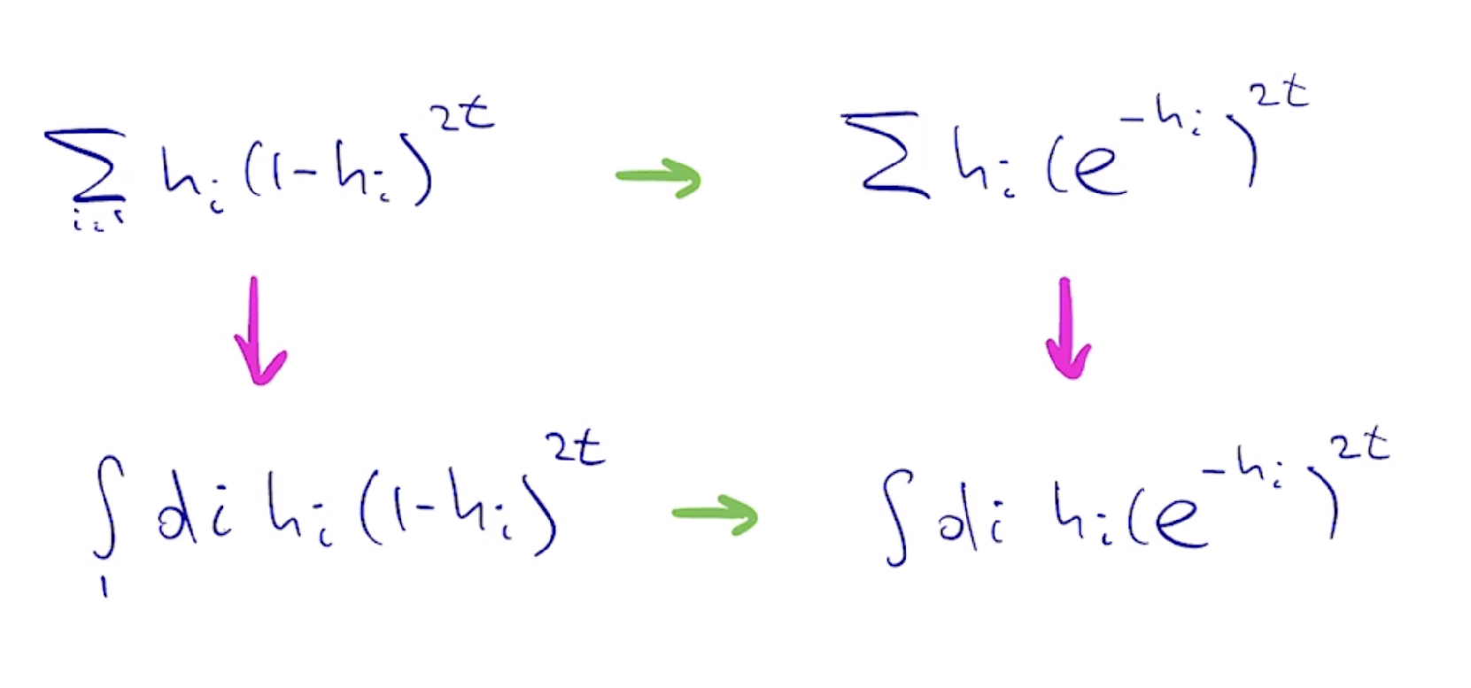
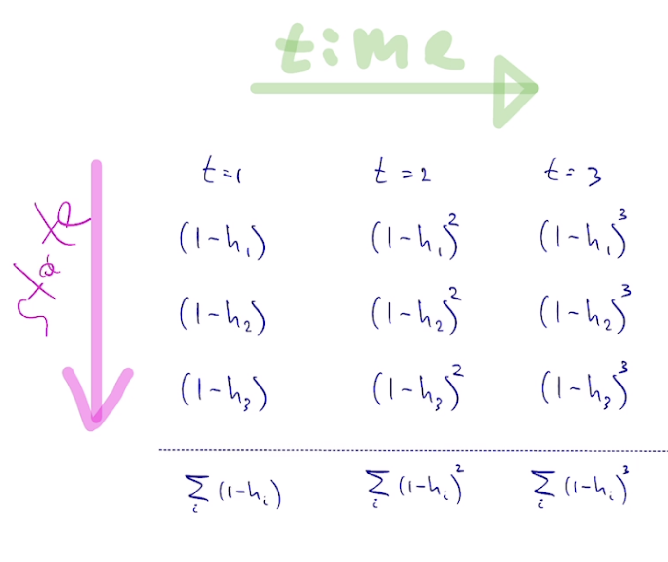
Four formulas below represent different ways of approximating f(t) I call the purple arrow “continuous state” approximation and green arrow “continuous time” approximation. Another way of viewing these two approximations:
Continuous time
Continuous time
For a 1-d quadratic, we have the following recurrence and continuous approximation--h-hw(t)We get corresponding closed form solutions using RSolve and DSolve
w
t+1
w
t
w
t
dw(t)
dt
In[]:=
RSolveValue[{w[t+1]==(1-h)w[t],w[0]==1},w[t],t]DSolveValue[{w'[t]==-hw[t],w[0]==1},w[t],t]
Out[]=
t
(1-h)
Out[]=
-ht
(TODO: plot)
DiscretePlot[]
-2
i
Caveat
Caveat
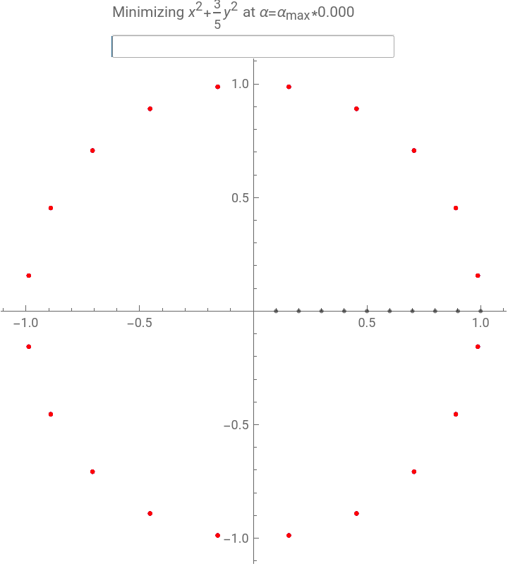
This analogy also extends to matrix valued H, in which case we get matrix power vs matrix exponential. This approximation becomes accurate in high dimensions when using step size 1/2 of “largest convergent”, the case in question. For divergent step sizes, gradient descent can diverge while continuous time approximation still converges, as you can see below.
Out[]=


Continuous state
Continuous state
We can replace sums over dimensions with an integral. Equivalently, we “smooth out” the jumps at individual points.
Out[]=
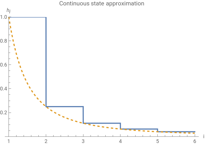


K.Grammatikos pointed out that we can use Euler-Maclaurin formula to bound the error of continuous state approximation. Take the special case of , we have

continuous space, discrete time, has a closed form solution in terms of Beta integral
Continuous time, continuous space:
Tool 2, change of variables
Tool 2, change of variables
We can simplify things further by absorbing h into the the density
Integral Transforms + Generating Functions
Moment-generating function
Moment-generating function
Write our sum as a density integral, then apply “continuous-time approximation”
To keep formulas simpler, do the 2t->t substitution, so the result is written in standard form for generating function
After applying “continuous-space approximation” from previous section, we get an integral equivalent to the moment generating function of Beta(1/2,1) distribution
We can plot this approximation against exact value of the loss for the first few steps
Integral Transforms
Integral Transforms
Now that our loss is written in terms of moment-generating function, we can apply Integral Transforms to obtain closed form solutions.
Below is the master diagram indicating how these transforms relate to each other
Below is the master diagram indicating how these transforms relate to each other
Laplace
Laplace
Get the formula by integrating over the density in [0..1] interval
We can turn it into Laplace transform, defined as integral over 0..∞ interval by multiplying by a constant function that’s 0 outside of 0..1 range
Stieltjes then reverse Laplace
Stieltjes then reverse Laplace
Compute Stieltjes transform
We can compute inverse Laplace Transform by expressing it in terms of inverse Mellin Transform, suggested by Mariusz in this post
Sequence Generating Functions
Sequence Generating Functions
frequency domain F(s) can be written as a sum over the sequence of moments
It is the ordinary generating function of this sequence
Likewise our time domain f(t) expression corresponds to the exponential generating function of this sequence