Legendre things
Dara O Shayda
dara@compclassnotes.com
March 1st 2025
dara@compclassnotes.com
March 1st 2025
Abstract
Legendre polynomials, differential equations and recurrence equations and many more computations useful to the author’s research are placed into this technical note for future reference. Symbolic computing scripts are added for every step of computations to serve as motivations for the unfamiliar readers. The note starts by computing the 1/r and r being distance between two points in 3D space. Moving forward, the scripts show how the Legendre “things” can provide effective tools for computing general solutions to the Laplacian equation. Furthermore, the interested readers could gain more insight by hands-on symbolic computing to understand the potential theory at large. The code in the technical code is based upon one of the most modern symbolic computing platforms, and yet even a STEM student can easily run the scripts in this note by copying and pasting from the PDF text or by accessing this persistent cloud object which contains the code:
https://www.wolframcloud.com/obj/ccn2/Published/Legendre_things.nb
Keywords: Laplace Equation, Whittaker, inverse distance potential, 1/r potential, Laplace ‘s Equation of Wave Motion, undulatory theory of gravity, symbolic computing, Legendre differential equation, Legendre recurrence equation, Legendre polynomials, surface harmonics, spherical harmonics, Rodrigues’ formula.
Software
Scripts: Symbolic computations performed in Wolfram Mathematica 14.2 .Notebook: https://www.wolframcloud.com/obj/ccn2/Published/Legendre_what.nb Support: Constant the author for additional code, bugs, correction in maths and so on.Nomenclature: Functions and most identifiers start with lower case letters, all native vendor identifiers start with upper case. No Packaging: There is no software engineering applied to the code here nor elsewhere in the author’s technical notes to reduce the difficulties and version mismatches in future. The eager readers can simply copy paste the code or download and run the notebook. TODO: 1. Algorithm details on the computing the recurrence equations for Legendre polynomials 2. Add the two variable recurrence equations for Legendre polynomials and custom derivations3. Actual model of a planetary gravity using the Legendre polynomials (NASA’s)4. Much larger and more detailed solutions to the Laplace equation for 1/r potentials via Legendre polynomials (Whittaker [1,3])5. How the Laplace’s equation is derived from assumptions about the flux© 2012-Present CCN StudiosCreative Commons Attribution-NonCommercial-ShareAlike 4.0

1.0 Conspectus
The Laplace’s Equation for scalar function V in rectangular coordinate system:
2
∂
∂
2
x
2
∂
∂
2
y
2
∂
∂
2
z
For brevity and without loss of generality the Harmonic Functions or Harmonics are scaler functions that satisfy the Laplace’s equation.
● c1: Existing potentials in spatial regions that do not contain mass nor electrical charges satisfy the Laplace’s equation. In general, Laplace’s equation describes situations of equilibrium, or those that do not depend explicitly on time. [4]
● c2: Legendre series is used for computing the 1/r and r being the distance between two points.
● c3: Using the computations from c2 Legendre’s series, differential equations and recurrence equations are derived, all in Symbolic computing scripts.
● c4: Many physical properties of the Earth, such as its magnetic field, are not azimuthal-symmetric about the rotation axis when examined in detail. However, these properties can be described using mathematical functions that are based upon the Legendre polynomials and series. [6]
● c5: Solutions
Remark 1.0.1: Variable separation assumption, indicating the three functions are independent of each other modulo a constant factor:
In[]:=
V=X[x]*Y[y]*Z[z]
Out[]=
X[x]Y[y]Z[z]
We cannot expect all solutions to Laplace’s equation to be of this simple, factorized form; the vast majority are not. The hope is that a superposition of factorized solutions will form the unique solution to a given boundary-value problem.
In[]:=
Expand[Laplacian[V,{x,y,z}]/V]
Out[]=
′′
X
X[x]
′′
Y
Y[y]
′′
Z
Z[z]
Set the Laplacian to 0:[x]+[y]+[z]=0Move the last two terms to the right hand side:[x]=-[y]-[z]The left hand side is entirely in X[x] while the right hand side is a mix of Y[y] and Z[z] which concludes X[x] is dependent on the other two functions and thus contradicts the separation of variables assumption see Remark 1.0.1.In order to avoid this contradiction the only possible way out is assuming the three rational functions are constants!
′′
X
X[x]
′′
Y
Y[y]
′′
Z
Z[z]
′′
X
X[x]
′′
Y
Y[y]
′′
Z
Z[z]
Assuming the rational functions are constant, set them to constant squares as below and solve the corresponding differential equations:
In[]:=
solX=DSolveValue[x]==-α^2,X[x],x,GeneratedParameters(Subscript[a,#]&)
′′
X
X[x]
Out[]=
Cos[xα]+Sin[xα]
a
1
a
2
Remark 1.0.2: Note that by assigning the generated parameters e.g. or to , the complex variables solutions are obtained.
a
1
a
2
In[]:=
solY=DSolveValue[y]==-β^2,Y[y],y,GeneratedParameters(Subscript[b,#]&)
′′
Y
Y[y]
Out[]=
Cos[yβ]+Sin[yβ]
b
1
b
2
In[]:=
solZ=DSolveValue[z]==α^2+β^2,Z[z],z,GeneratedParameters(Subscript[c,#]&)
′′
Z
Z[z]
Out[]=
z+
2
α
2
β
c
1
-z+
2
α
2
β
c
2
Multiply the solutions to compute the V:
In[]:=
solX*solY*solZ
Out[]=
(Cos[xα]+Sin[xα])(Cos[yβ]+Sin[yβ])+
a
1
a
2
b
1
b
2
z+
2
α
2
β
c
1
-z+
2
α
2
β
c
2
Check if the latter satisfies the Laplace’s equation:
In[]:=
FullSimplify@Laplacian[solX*solY*solZ,{x,y,z}]
Out[]=
0
2.0 1/r series
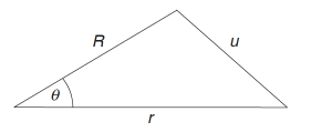
● Let r and R be the sides of a triangle that enclose an angle θ and let u be the side
opposite this angle (Fig. 2.0.1). The angle and sides are related by the cosine rule:
=+-2rRCos[θ]
opposite this angle (Fig. 2.0.1). The angle and sides are related by the cosine rule:
2
u
2
r
2
R
In[]:=
Clear[u];sol=Normal@Solve[u^2==r^2+R^2-2*r*R*Cos[θ],{u},Reals]
Out[]=
u-+-2rRCos[θ],u+-2rRCos[θ]
2
r
2
R
2
r
2
R
Fig. 2.0.1
● Set u to the positive solution of the cosine rule:
In[]:=
Clear[u];u=u/.sol[[2]][[1]]
Out[]=
2
r
2
R
● Square the solution namely and do some, not really obvious, replacements to compute:
2
u
Cos[θ]→x
r→Rh
(h^2-2*h*x)→-t
In[]:=
Simplify[((u^2/.{r->R*h,Cos[θ]->x}))/R^2]/.{(h^2-2*h*x)->-t}
Out[]=
1-t
such that = (Eq. 2.0.2)Note that = .The replacements reduced the to 1-t .
1
u
1
R
1
(1-t)
1
(1-t)
1
1+-2hx
2
h
2
u
● Define a Binomial term in a power series for variable t: (see [7])
In[]:=
(*(x+y)^rwithkiteratorinteger,rcanbeanyrealnumber*)binomialTerm[x_,y_,r_,k_]:=(FactorialPower[r,k]/k!)*x^(r-k)*y^k;
Take a look at the output:
In[]:=
binomialTerm[1,(-t),-1/2,3]
Out[]=
5
3
t
16
Compute manually to get a feel:
In[]:=
(-1/2)*(-1/2-(3-1))*(-1/2-(2-1))/3!
Out[]=
-
5
16
Note that the -t to the odd powers produces a -1 factor thus all terms have positive rational numbers as coefficients.
Follow the rest of steps required to complete the derivation of (EQ 2.0.3):
● Collect and sort the coefficients for the variable/symbol h, which are mostly polynomials in x:
● Collect and sort the coefficients lists for the variable/symbol h which are polynomials in x:
● Use (Eq. 2.0.2) to compute the series for 1/u:
● Format and output as String:
2.1 Legendre Differential Equation
● Computations below fit the ψ to a differential equation as follows.
● Replace
The last output is the left hand side of the differential equation:
Recall (Eq. 2.2.1)
This is coined as Legendre differential equation. It has a family of solutions, each of which is a polynomial corresponding to a particular value of integer n. The Legendre polynomials provide solutions in potential analyses with spherical symmetry, and have an important role in geophysical theory.
Let us use the Leibniz’s rule to repeatedly compute the derivative of certain polynomials.
ϱ is a replacement rule for typesetting:
Repeatedly derivate u[x] v[x], notation is for typesetting and brevity:
● By induction or other methods one can easily generalize the above computations:
Start with function f(x):
● Differentiating f(x) once with respect to x gives
● This is a recurrence equation:
Formal symbols can be temporarily modified inside a Block because Block clears all definitions associated with a symbol, including Attributes. Table works essentially like Block, thus also allowing temporary changes.
● Case1
● Case2
3.0 Laplace solutions
Legendre polynomials satisfy the Laplacian equation. They are more than often used in combination with others such as SphericalHarmonicY[ ] and BesselJ[ ].
Furthermore they are indispensable part of time varying Laplacian wave motion equations.
Furthermore they are indispensable part of time varying Laplacian wave motion equations.
3.1 Time independent: Surface Harmonics
3.1.1 Enter The Surface Harmonics!
Let us use the SphericalPlot3D[ ], but before embarking simply plot constant 1 in the spherical plot. As you can view the plot turns out to be a Sphere of radius one and that makes all the sense:
It is difficult to plot the wave structure of the Legendre Polynomial solutions to the time independent Laplace equation (and we tried!!!), however we can plot these waves on the surface of a Sphere by merely adding r or better numeral 1 to the potential!
Thus the name: Surface Harmonic, namely periodic functions on the boundary of Sphere for visualization of the solutions.
Thus the name: Surface Harmonic, namely periodic functions on the boundary of Sphere for visualization of the solutions.
Exaggerated Surface Harmonics using Spherical Plot by overly scaling the periodic Legendre polynomial solution on surface of Sphere of radius 1 (the 1 + ...) :
And you have seen these plots [8, 10]:
Earth’s gravity measured by NASA GRACE mission, showing deviations from the theoretical gravity of an idealized, smooth Earth, the so-called Earth ellipsoid. Red shows the areas where gravity is stronger than the smooth, standard value, and blue reveals areas where gravity is weaker.
Earth’s gravity measured by NASA GRACE mission, showing deviations from the theoretical gravity of an idealized, smooth Earth, the so-called Earth ellipsoid. Red shows the areas where gravity is stronger than the smooth, standard value, and blue reveals areas where gravity is weaker.
3.1.2 The sum of Surface Harmonics is again Surface Harmonic!
3.2 Time dependent: The equation of wave motions
This equation is of general occurrence in investigations of undulatory disturbances propagated with velocity c independent of the wave length; for example, in the theory of electric waves and the electro-magnetic theory of light, it is the equation satisfied by each component of the electric or magnetic vector; in the theory of elastic vibrations, it is the equation satisfied by each component of the displacement; and in the theory of sound, it is the equation satisfied by the velocity potential in a perfect gas.[3]
● Compute a potential by multiplying Legendre polynomial and BesselJ[ ]:
● Test for Laplacian Equation:
● Compute the Re
● Transform the potential to Cartesian coordinates to plot and animate:
● In the following time-framed animation sequence, shortly after time 0 disturbance appears and continues gaining amplitude and as can be viewed quite wave-like. The disturbance dies off and again picks up amplitude and continues.
References
[1] E.T Whittaker , On the Partial Differential Equations of Mathematical Physics, Mathematische Annalen Vol 57, 1903, p. 333-355
[2] Jeremy Dunning-Davies, Some Important Neglected Equations of Physics.
https://vixra.org/pdf/2007.0002v1.pdf
[3] E.T Whittaker , Watson , A Course of Modern Analysis, Fifth Edition ,ISBN 978-1-316-51893-9
[4] https://en.wikipedia.org/wiki/Laplace%27s_equation
[5] https://en.wikipedia.org/wiki/Legendre_polynomials
[6] W. Lowrie, A Student’s guide to Geophysical Equations , Cambridge University Press, New York
[7] https://en.wikipedia.org/wiki/Binomial_theorem#Newton’s_generalized_binomial_theorem
[8] https://en.wikipedia.org/wiki/Gravity_of_Earth
[9] https://en.wikipedia.org/wiki/Geopotential_spherical_harmonic_model
[10] E. Sinem Ince, Franz Barthelmes, ICGEM – 15 years of successful collection and distribution of global gravitational models, associated services, and future plans:
https://www.researchgate.net/publication/333132180_ICGEM_-_15_years_of_successful_collection_and_distribution_of_global_gravitational_models_associated_services_and_future_plans