Legendre things
Dara O Shayda
dara@compclassnotes.com
March 1st 2025
dara@compclassnotes.com
March 1st 2025
Abstract
Legendre polynomials, differential equations and recurrence equations and many more computations useful to the author’s research are placed into this technical note for future reference. Symbolic computing scripts are added for every step of computations as motivations for the unfamiliar readers. The note stars by computing the 1/r and r being distance between two points in 3D space. Moving forward scripts show how the Legendre “things” can provide effective tools for computing general solutions to the Laplacian equation. The code in the technical code is based upon one of the most modern symbolic computing platforms, and even a STEM student can easily run the scripts in this note by copying and pasting PDF text or by accessing this persistent cloud object which contains the code:
Software
Scripts: Symbolic computations performed in Wolfram Mathematica 14.2 .TODO: © 2012-Present CCN StudiosCreative Commons Attribution-NonCommercial-ShareAlike 4.0

1.0 Conspectus
The Laplace’s Equation for scalar function V in rectangular coordinate system:
2
∂
∂
2
x
2
∂
∂
2
y
2
∂
∂
2
z
For brevity and without loss of generality the Harmonic Functions or Harmonics are scaler functions that satisfy the Laplace’s equation.
● c1: Existing potentials in spatial regions that do not contain mass or electrical charges satisfy the Laplace’s equation. In general, Laplace’s equation describes situations of equilibrium, or those that do not depend explicitly on time. [4]
● c2: Legendre series is used for computing the 1/r and r bring the distance between two points.
● c3: Using the computations from c2 Legendre’s series, differential equations and recurrence equations are derived, all in scripts.
● c4: Many physical properties of the Earth, such as its magnetic field, are not azimuthal-symmetric about the rotation axis when examined in detail. However, these properties can be described using mathematical functions that are based upon the Legendre polynomials and series. [6]
2.0 1/r series
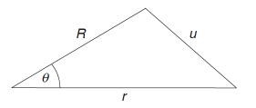
● Let r and R be the sides of a triangle that enclose an angle θ and let u be the side
opposite this angle (Fig. 2.0.1). The angle and sides are related by the cosine rule:
=+-2*r*R*Cos[θ]
opposite this angle (Fig. 2.0.1). The angle and sides are related by the cosine rule:
2
u
2
r
2
R
In[]:=
Clear[u];sol=Normal@Solve[u^2==r^2+R^2-2*r*R*Cos[θ],{u},Reals]
Out[]=
u-+-2rRCos[θ],u+-2rRCos[θ]
2
r
2
R
2
r
2
R
Fig. 2.0.1
● Set u to solution to the cosine rule:
In[]:=
Clear[u];u=u/.sol[[2]][[1]]
Out[]=
2
r
2
R
● Square solution and do some not really obvious replacements to compute:
2
u
In[]:=
Simplify[((u^2/.{r->R*h,Cos[θ]->x}))/R^2]/.{(h^2-2*h*x)->-t}
Out[]=
1-t
such that = (Eq. 2.0.2)
1
u
1
R
1
(1-t)
Define a term in a series for variable t:
Clear[k];binomialTerm[x_,y_,r_]:=Binomial[r,k]*x^(r-k)*y^k;
Take a look at the output:
In[]:=
binomialTerm[1,(-t),-1/2]
Out[]=
k
(-t)
1
2
In[]:=
Sum[binomialTerm[1,(-t),-1/2],{k,0,5}]
Out[]=
1+++++
t
2
3
2
t
8
5
3
t
16
35
4
t
128
63
5
t
256
In[]:=
series=Sum[binomialTerm[1,(-t),-1/2],{k,0,5}]/.{t->(-(h^2-2*h*x))}
Out[]=
1+(-+2hx)++++
1
2
2
h
3
8
2
(-+2hx)
2
h
5
16
3
(-+2hx)
2
h
35
128
4
(-+2hx)
2
h
63
256
5
(-+2hx)
2
h
In[]:=
Collect[series,h]
Out[]=
1-+hx++-+-++-++-++-+-+-++-+
63
10
h
256
315x
9
h
128
8
h
35
128
315
2
x
32
2
h
1
2
3
2
x
2
3
h
3x
2
5
3
x
2
7
h
35x
16
315
3
x
16
6
h
5
16
105
2
x
16
315
4
x
16
4
h
3
8
15
2
x
4
35
4
x
8
5
h
15x
8
35
3
x
4
63
5
x
8
In[]:=
xcoeff=CoefficientList[series,h]
Out[]=
1,x,-+,-+,-+,-+,-+-,-+,-,,-
1
2
3
2
x
2
3x
2
5
3
x
2
3
8
15
2
x
4
35
4
x
8
15x
8
35
3
x
4
63
5
x
8
5
16
105
2
x
16
315
4
x
16
35x
16
315
3
x
16
35
128
315
2
x
32
315x
128
63
256
In[]:=
legendrePn=xcoeff/.{x->Cos[θ]}
Out[]=
1,Cos[θ],-+,-+,-+,-+,-+-,-+,-,,-
1
2
3
2
Cos[θ]
2
3Cos[θ]
2
5
3
Cos[θ]
2
3
8
15
2
Cos[θ]
4
35
4
Cos[θ]
8
15Cos[θ]
8
35
3
Cos[θ]
4
63
5
Cos[θ]
8
5
16
105
2
Cos[θ]
16
315
4
Cos[θ]
16
35Cos[θ]
16
315
3
Cos[θ]
16
35
128
315
2
Cos[θ]
32
315Cos[θ]
128
63
256
In[]:=
invuSeries=Table[((r/R)^(i-1))*legendrePn[[i]],{i,1,Length@legendrePn}]/R
Out[]=
,,-+,-+,-+,-+,-+-,-+,-,,-
1
R
rCos[θ]
2
R
2
r
1
2
3
2
Cos[θ]
2
3
R
3
r
3Cos[θ]
2
5
3
Cos[θ]
2
4
R
4
r
3
8
15
2
Cos[θ]
4
35
4
Cos[θ]
8
5
R
5
r
15Cos[θ]
8
35
3
Cos[θ]
4
63
5
Cos[θ]
8
6
R
6
r
5
16
105
2
Cos[θ]
16
315
4
Cos[θ]
16
7
R
7
r
35Cos[θ]
16
315
3
Cos[θ]
16
8
R
8
r
35
128
315
2
Cos[θ]
32
9
R
315Cos[θ]
9
r
128
10
R
63
10
r
256
11
R
Use (Eq. 2.0.2) to compute the series for 1/u:
In[]:=
Row@{"1/u"," = ","(1/R)","(",Total@Table[Row@{If[i>1,(("(r/R)")^(i-1)),Nothing],legendrePn[[i]]},{i,1,Length@legendrePn}],")"}
Out[]=
1/u = (1/R)(1+(r/R)Cos[θ]+-++-++-++-++-+-+-++-++-)
2
(r/R)
1
2
3
2
Cos[θ]
2
3
(r/R)
3Cos[θ]
2
5
3
Cos[θ]
2
4
(r/R)
3
8
15
2
Cos[θ]
4
35
4
Cos[θ]
8
5
(r/R)
15Cos[θ]
8
35
3
Cos[θ]
4
63
5
Cos[θ]
8
6
(r/R)
5
16
105
2
Cos[θ]
16
315
4
Cos[θ]
16
7
(r/R)
35Cos[θ]
16
315
3
Cos[θ]
16
8
(r/R)
35
128
315
2
Cos[θ]
32
9
(r/R)
315Cos[θ]
128
10
(r/R)
63
256
r/R < 1 condition for convergence
2.1 Differential Equation
In[]:=
ψ=(1-2*x*h+h^2)^(-1/2)
Out[]=
1
1+-2hx
2
h
In[]:=
ϱ={(1+-2hx)->Hold[ψ]^-2};
2
h
In[]:=
dhψ=FullSimplify@PowerExpand[(ψ)/.ϱ]
∂
h
Out[]=
(-h+x)
3
Hold[ψ]
In[]:=
dxψ=FullSimplify@PowerExpand[(ψ)/.ϱ]
∂
x
Out[]=
h
3
Hold[ψ]
In[]:=
dxxψ=ψ
∂
x,x
Out[]=
3
2
h
5/2
(1+-2hx)
2
h
In[]:=
dxxψ=PowerExpand[ψ/.ϱ]
∂
x,x
Out[]=
3
2
h
5
Hold[ψ]
In[]:=
dhψ=Simplify@PowerExpand[((h*ψ))/.ϱ]
∂
h
Out[]=
Hold[ψ]+h(-h+x)
3
Hold[ψ]
In[]:=
dhhψ=Simplify/@Collect[Expand@PowerExpand[(h*ψ)/.ϱ],Hold[ψ]]
∂
h,h
Out[]=
(-3h+2x)+3h
3
Hold[ψ]
2
(h-x)
5
Hold[ψ]
In[]:=
dhhψ2=dhhψ/.{->Hold[dxψ]h,->Hold[dxxψ](3*h^2)}
3
Hold[ψ]
5
Hold[ψ]
Out[]=
2
(h-x)
h
(-3h+2x)Hold[dxψ]
h
(Eq. 2.2.1)
This is the Legendre differential equation. It has a family of solutions, each of which is a polynomial corresponding to a particular value of n. The Legendre polynomials provide solutions in potential analyses with spherical symmetry, and have an important role in geophysical theory.
2.2 Polynomial Series
The Legendre polynomials Pn(x) are defined in (1.156) as the coefficients of hn in the expansion of Ψ as a power series. On multiplying both sides of (1.156) by h, we get
Recall (Eq. 2.2.1)
2.3 Recurrence Equation
(1:218) p 43 student
3.0 Laplace solutions
References
[1] E.T Whittaker , On the Partial Differential Equations of Mathematical Physics, Mathematische Annalen Vol 57, 1903, p. 333-355
[2] Jeremy Dunning-Davies, Some Important Neglected Equations of Physics.
https://vixra.org/pdf/2007.0002v1.pdf
[3] E.T Whittaker , Watson , A Course of Modern Analysis, Fifth Edition ,ISBN 978-1-316-51893-9
[4] https://en.wikipedia.org/wiki/Laplace%27s_equation
[5] https://en.wikipedia.org/wiki/Legendre_polynomials
[6] W. Lowrie, A Student’s guide to Geophysical Equations , Cambridge University Press, New York