In[]:=
Fri 26 May 2023 15:33:19
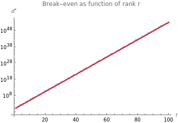
Break-even point for infinite rank
Break-even point for infinite rank
Question: For which d does resemble the infinite dimensional version in terms of effective rank?Answer: for d>/exp(γ)
1^-p,2^-p,3^-p,...,
-p
d
1
p-1
(2+
2
)math.SE question:
- Smallest value of d such that (math.SE post)
- Getting a series expansion for implicitly defined function (mathematica.SE post)
Other notebooks:
- alpha-capacity-effective-rank.nb
- Smallest value of d such that (math.SE post)
- Getting a series expansion for implicitly defined function (mathematica.SE post)
Other notebooks:
- alpha-capacity-effective-rank.nb
TLDR;
- Claude turns it into continuous root finding problem, using continuous generalization of Harmonic number
- Gary gives simpler version of Harmonic in terms of Zeta/truncated sum
- Michael E2 fixes Plot bug, need to use SetPrecision
- Claude turns it into continuous root finding problem, using continuous generalization of Harmonic number
- Gary gives simpler version of Harmonic in terms of Zeta/truncated sum
- Michael E2 fixes Plot bug, need to use SetPrecision
In[]:=
Clear["Globals`*"];predict[p_]:=Exp-0.5843521872961219`+1.228079016227338`*;breakEven[p_]:=d/.FindRoot==*2,{d,Floor[predict[p]]},AccuracyGoal->1rvals=Table[r,{r,1.,100}];dvals=breakEven[1+1/#]&/@rvals;observedPlot=ListPlot[{rvals,dvals},ScalingFunctions->{Automatic,"Log"},AxesLabel->{"r",""},PlotLabel->"Break-even as function of rank r",PlotLegends->{"observed"}];fit=LinearModelFit[{rvals,Log@dvals},x,x]predictedPlot=LogPlot[Exp@fit[r],{r,Min@rvals,Max@rvals},PlotLegends->{fit},PlotStyle->Red];Show[observedPlot,predictedPlot]
1
p-1
2
Zeta[p]
Zeta[2p]
2
Sum[,{i,1,d}]
-p
i
Sum[,{i,1,d}]
-2p
i
*
d

15
10
16
10
16
10
Out[]=
FittedModel
Out[]=
In[]:=
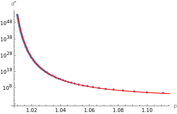
predict2[p_]:=Exp-0.5872825625315911`+1.2281342999064533`;pvals=Table1+,{r,2.,100};dvals=breakEven/@pvals;sf={Automatic,"Log"};observedPlot=ListPlot[{pvals,dvals},ScalingFunctions->sf,PlotStyle->PointSize[Medium]];predictedPlot=Plot[predict2[p],{p,Min[pvals],Max[pvals]},PlotRange->All,ScalingFunctions->sf,PlotLegends->{MaTeX["c_1 \\exp \\left(\\frac{c_2}{p-1}\\right)"]},PlotStyle->Red];Show[observedPlot,predictedPlot,AxesLabel->{"p",""}]
1
p-1
1
r
*
d
15
10
16
10
16
10
Out[]=

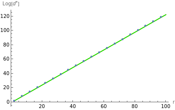
Use Claude and Gary approximation
Use Claude and Gary approximation
In[]:=
(*ClaudeVersion*)asymp1[p_]:=(f[x_]:=Log[2Zeta[2p]]-Log[HarmonicNumber[Exp[x],2p]];x/.FindRoot[f[x],{x,10},WorkingPrecision->20]);(*GaryapproximationofHarmonicnumber*)harmonicNumber[d_,p_]:=Zeta[p]-;asymp2[p_]:=(f[x_]:=Log[2Zeta[2p]]-Log[harmonicNumber[Exp[x],2p]];x/.FindRoot[f[x],{x,10},WorkingPrecision->20]);rvals=Table[r,{r,2,100,5}];pvals=Table1+,{r,rvals};dvals1=asymp1/@pvals;dvals2=asymp2/@pvals;data1={rvals,dvals1};data2={rvals,dvals2};linearFit1=LinearModelFit[data1,x,x];linearFit2=LinearModelFit[data2,x,x];fittedPlot1=Plot[linearFit1[x],{x,2,100},PlotStyle->Red];fittedPlot2=Plot[linearFit2[x],{x,2,100},PlotStyle->Green];observedPlot1=ListPlot[data1];observedPlot2=ListPlot[data2,PlotStyle->PointSize[Small]];Show[fittedPlot1,fittedPlot2,observedPlot1,AxesLabel->{"r","Log[]"}]
2
HarmonicNumber[Exp[x],p]
2
Zeta[p]
1-p
d
p-1
2
harmonicNumber[Exp[x],p]
2
Zeta[p]
1
r
*
d
Out[]=
In[]:=
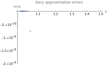
ListPlot[{pvals,dvals1-dvals2},ScalingFunctions->{"Log",Automatic},PlotLabel->"Gary approximation errors",AxesLabel->{"p","error"}]
Out[]=
Simpler plot
Simpler plot
In[]:=
ClearAll["Globals`*"];g[r_,x_]=Log2Zeta21+-Log-+Zeta21+;f[r_]:=x/.FindRoot[g[r,x],{x,1}];Plot[f[r],{r,1,10},AxesLabel->{"r","f(r)"}]
2
-r+Zeta1+
-1/r
()
x
1
r
1
r
2
Zeta1+
1
r
1-21+
1
r
()
x
-1+21+
1
r
1
r
Roman answer
Roman answer
Relative error of Roman’s approximation
Relative error of Roman’s approximation
Asymptotic Inversion general approach
Asymptotic Inversion general approach