In[]:=
Thu 23 Nov 2023 12:37:54
- math.SE question “Distribution of k’th squared singular value of a Gaussian matrix?“ post
- SF ML presentation mlc-norms-present.nb
- SF ML presentation mlc-norms-present.nb
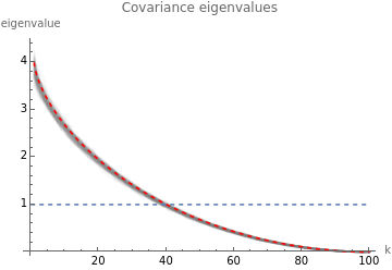
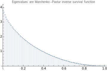
Distribution of eigenvalues
Distribution of eigenvalues
Out[]=
Out[]=
Out[]=
In[]:=
SUPERHUGE`SUPERHUGE=1;
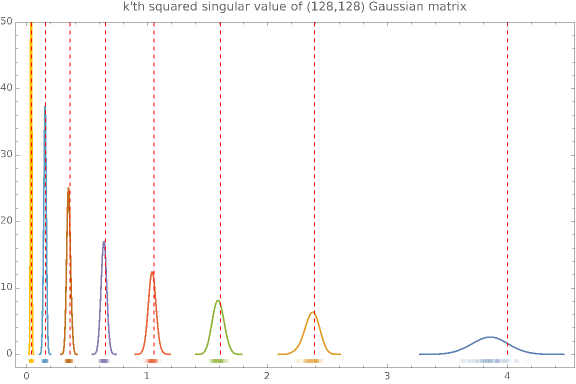
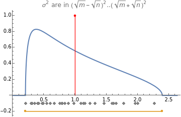
Limits of Marchenko-Pastur
Limits of Marchenko-Pastur
In[]:=
(*nobservations,mfeatures*)colors=ColorData[97,"ColorList"];numSamples=100;m=30;n=100;(*Normalizetohaveobservationshavesquarednorm1onaverage*)xs0=RandomVariate[NormalDistribution[],{m,n}],numSamples]];(*RangeofMarchenkoPasturforeigsofXX/n*)minRange=n;maxRange=n;numberPlot=NumberLinePlot[{svals2,Interval[{minRange,maxRange}]},Spacings->-0.1,PlotStyle->{Gray,colors[[2]]},PlotLegends->{"observed","ESD bounds"}];esdPlot=Plot[PDF[MarchenkoPasturDistribution[m/n],x],{x,0,1.1*maxRange},PlotStyleThick,ExclusionsNone,PlotRange->All];meanPlot=ListPlot[{{1,1}},Filling->Axis,FillingStyle->Red,PlotStyle->Red,PlotRange->{0,1},PlotLegends->{"mean"}];Show[esdPlot,numberPlot,meanPlot,PlotRange->All,PlotLabel->" are in .."]
n
;svals2=Flatten[Table[2
(SingularValueList@xs0)
2
m
-n
2
m
+n
2
σ
m
-n
2
)\),
m
+n
2
)\),
Out[]=
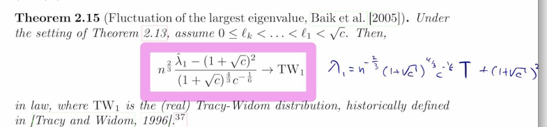
Tracy-Widom
Tracy-Widom
From “Couillet, Romain, and Zhenyu Liao. 2022. Random Matrix Methods for Machine Learning. Cambridge, England: Cambridge University Press.”
In[]:=
Clear[c,n];formula0=;
2/3
n0
lambda-
2
1+
c0
4/3
1+
c0
-1/6
c0
In[]:=
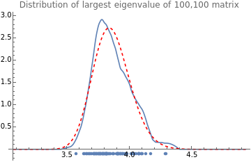
numSamples=100;m=100;n=100;c=m/n;numSamples=100;formula=formula0/.{n0->n,c0->c};expr=First@SolveValues[formula==z,lambda];twDensity=PDF[TransformedDistribution[expr,zTracyWidomDistribution[1]],x];randmat:=With[{X=RandomVariate[NormalDistribution[],{n,n}]},X.X/n];norms=Table[Norm[randmat],{numSamples}];boundedPDF[vals_,bounds_,var_]:=PDF[SmoothKernelDistribution[vals,Automatic,{"Bounded",bounds,"Epanechnikov"}],var];minRange=n;maxRange=n;bounds=maxRange-,maxRange+;fittedDensity=boundedPDF[norms,bounds,x];densityPlot=Plot[{fittedDensity,twDensity},{x,bounds[[1]],bounds[[2]]},PlotLegends->{"empirical density","Tracy-Widom"},PlotRange->All,PlotStyle->{Automatic,Directive[Red,Dashed]}];numberPlot=NumberLinePlot[{norms},Spacings->{-.1},PlotLegends->{"observed norms"}];Show[densityPlot,numberPlot,PlotLabel->SF["Distribution of largest eigenvalue of ``,`` matrix",m,n]]
2
m
-n
2
m
+n
2
1/6
n
2
1/6
n
Out[]=
Tracy-Widom mean
Tracy-Widom mean