In[]:=
Fri 1 Dec 2023 16:30:42
Cleaned up verson in scratch-matrix-growthTLDR Nov 24: for unit frobenius norm matrix, multiplying by dimension keeps L2 norm constant, multipying by keeps Linf norm constant.When going backwards, there’s growth either way, probably due to correlations, on second pass, vectors are more adversarial
input
output
Init
Init
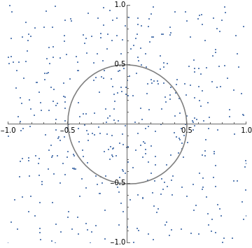
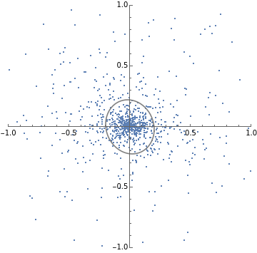
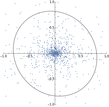
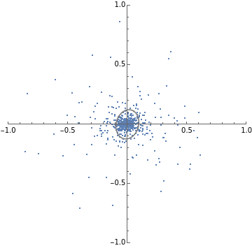
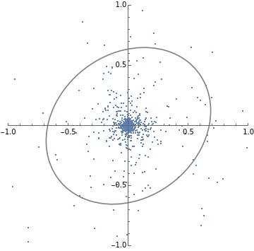
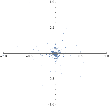
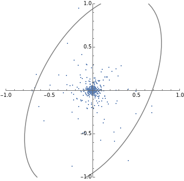
SGD Trajectory plots
SGD Trajectory plots
In[]:=
SeedRandom[1];batchStepDist[W_,α_]:=Module[{},step[x_,w_]:=Module[{},(IdentityMatrix[d]-αOuter[Times,x,x]).w];MapThread[step,{RandomVariate[dist,n],W}]];stepL2SGDfast[h_]:=Module[{d=Length[h],normalize,step,evec},normalize[v_]:=v/Sqrt@Total[v*v];step[v_]:=2h*v+h*Total[v];evec=FixedPoint[normalize[step[#]]&,ConstantArray[1.,d],1000];2/Norm[step@evec]];h={1,3};d=Length[h];n=1000;numSteps=30;dist=MultinormalDistribution[{0,0},DiagonalMatrix[h]];W=RandomVariate[MultinormalDistribution[{0,0},DiagonalMatrix[{1,1}]],n];criticalAlpha=stepL2SGDfast[h];trajectories1=NestList[batchStepDist[#,criticalAlpha]&,W,numSteps];(*numStepsxBxdims*)trajectories2=NestList[batchStepDist[#,criticalAlpha*1.3]&,W,numSteps];(*numStepsxBxdims*)Print[stepL2SGDfast[h]]plots1=ListPlot[#,PlotRange{{-1,1},{-1,1}},AspectRatio1]&/@trajectories1[[;;;;10]];plots2=ListPlot[#,PlotRange{{-1,1},{-1,1}},AspectRatio1]&/@trajectories2[[;;;;10]];TableForm[{plots1,plots2}];(*Givencovariancematrix,plotcontourlinesthatalignedwithdata*)visualizeCov[cov_]:=Module{x,y},ContourPlot
{x,y}.PseudoInverse[cov].{x,y}
==.5,{x,-1,1},{y,-1,1},ContourStyle->Gray,ContourShading->None;getCov[data_]:=data.data/Length[data];(*visualizeCov@getCov@#&/@trajectories1[[;;;;10]]*)Print[stepL2SGDfast[h]]plots1=Show[ListPlot[#,PlotRange{{-1,1},{-1,1}},AspectRatio1],visualizeCov@getCov@#]&/@trajectories1[[;;;;10]];plots2=Show[ListPlot[#,PlotRange{{-1,1},{-1,1}},AspectRatio1],visualizeCov@getCov@#]&/@trajectories2[[;;;;10]];TableForm[{plots1,plots2}]0.211325
0.211325
Out[]//TableForm=

Norm growth/decay trajectories
Norm growth/decay trajectories
Linear simulation
Linear simulation
In[]:=
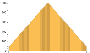
Print["up-down"];BarChart[upDownDims]simulate[upDownDims,randGaussian,normalizeFrob2,linearStep,1]smoothHistogram[]&/@takeEvenly[xs,5]Print["down-up"];BarChart[downUpDims]simulate[downUpDims,randGaussian,normalizeFrob2,linearStep,1]smoothHistogram[]&/@takeEvenly[xs,5]Print["constant"];BarChart[constantDims]simulate[constantDims,randGaussian,normalizeFrob2,linearStep,1]decreasingHistogram[]&/@takeEvenly[xs,5]
2
SingularValueList[#]
2
SingularValueList[#]
2
SingularValueList[#]
up-down
Out[]=
Out[]=
Visualize point trajectories
Visualize point trajectories
Centered ReLU simulation
Centered ReLU simulation