In[]:=
Tue 7 Nov 2023 15:30:28
Helper utilities
Helper utilities
Also run gs-vs-sgd init cells.
Utilities here are more specific to presentation/visualization.
Generic numerical analysis utilities useful outside of blogpost go to gd-vs-sgd
Utilities here are more specific to presentation/visualization.
Generic numerical analysis utilities useful outside of blogpost go to gd-vs-sgd
In[]:=
(*On[Assert];*)(* CircleTimes=KroneckerProduct;*)initSpectrum[h0_]:=(h=N@h0;d=Length[h];c0=ConstantArray[1.,d];);randomBasis[n_,k_]:=Module[{M,z,q,r,d,ph},z=RandomVariate[NormalDistribution[0,1],{n,n}];{q,r}=QRDecomposition[z];d=Diagonal[r];ph=d/Abs[d];M=q*ph;M[[;;k]]//Transpose];visualizeTrajectory[traj_]:=Module[{contour,bound},SeedRandom[2];basis=randomBasis[Length[h],2];bound=1;contour=ContourPlot@@{Total[(basis.{x,y})*h*(basis.{x,y})],{x,-bound,bound},{y,-bound,bound},ContourShadingNone,ContourStyleBlue};Show[contour,Graphics[{Arrowheads[Small],drawArrows[#.basis&/@traj]}]]];drawArrows[points_]:=(pairs=Partition[points,2,1];Arrow[pairs]);vec[W_]:=Transpose@{Flatten@Transpose[W]};unvec[Wf_]:=Module[{d},d=Sqrt[Dimensions[Wf]//First];Assert[dFloor[d]];Assert[d*dFirst@Dimensions[Wf]];unvec[Wf,d]];unvec[Wf_, rows_]:=Transpose[Flatten/@Partition[Wf,rows]];(* Gaussian sampler *)gaussianSampler[diag_]:=With{d=Length[diag]},Compile{{n,_Integer}},Module{vals},vals=
diag
*#&/@RandomVariate[NormalDistribution[],{n,d}];(*CircleTimes=KroneckerProduct;*)norm2[x_]:=Total@Flatten[x*x];signNormalize[vec_]:=vec*Sign[Total[vec]];SF=StringForm;Convergence + eigenvec animations of T
Convergence + eigenvec animations of T
forum-high-dimensional-trajectories.nb
gaussian-formulas.nb
gaussian-formulas.nb
In[]:=
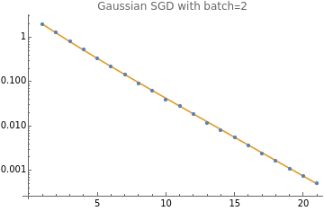
debugSampler[B_]:=Module[{},{{Sqrt[2],0},{0,2}}];(*batchweightedharmonicmeanbetweenminandmax.Suchthatb=1givesminandb=∞givesmax.Halfwaypointisat+1*)hmean[min_,max_,b_]:=+;cov[X_]:=X.X/Length[X];Clear[step,batchStep];h={1,2};d=Length[h];(*dimensions*)b=2;(*batchsize*)sampler=gaussianSampler[h];r=;(*effectiverankr*)rs=Witha=,b=1,+2;(*stochasticrankr,0.5ofharmonicmeanofr/2and1*)α=hmean[rs,r,b];α/=2;outer2[x_]:=Outer[Times,x,x];CircleTimes=KroneckerProduct;H=DiagonalMatrix[h];hh=outer2[h];II=IdentityMatrix[d];T=II-2αH+(2H.H+h⊗h)+H.H;SeedRandom[1];bound=1.2;numSteps=20;numSamples=2000;eb0=A.A.w;batchStep[wb_]:=step/@wb;ebHist=NestList[batchStep,eb0,numSteps];covHist=NestList[T.#&,ConstantArray[1.,d],numSteps];ListLogPlot[{Tr[cov@#]&/@ebHist,Tr/@covHist},PlotLegends->{"observed","predicted"},PlotStyle->{Small,Large},Joined->{False,True},PlotLabel->StringForm["Gaussian SGD with batch=``",b]]
max
min
b
1
min
b-1
max
Total[h]
Max[h]
r
2
2
1
a
1
b
2
Total[h]
2
α
1
b
b-1
b
2
CirclePoints[numSamples]//N;(*identitycovariance*)step[w_]:=With{A=sampler[b]},w-α
b
Out[]=
Near diagonal nature of operator
Near diagonal nature of operator
For large b, operator becomes diagonal, easy to approximate sum of entries with Trace.
https://www.wolframcloud.com/obj/yaroslavvb/nn-linear/forum-rank1-trace-user8675309.nb
https://www.wolframcloud.com/obj/yaroslavvb/nn-linear/forum-rank1-trace-user8675309.nb
How minimization happens in rotated coords
How minimization happens in rotated coords
Notation workout
Notation workout
Linked from blog: trajectories notability
https://notability.com/n/1IYM6pF2tCyAvfPRBANQPr
https://notability.com/n/1IYM6pF2tCyAvfPRBANQPr
Notation util
Notation util
Main
Main
Run blog-trajectories-util.nb
Fourth order moment check
Fourth order moment check