Quantum Linear Solvers
Quantum Linear Solvers
Solving linear systems is at the heart of countless applications, from physics simulations to machine learning. In quantum computing, the Quantum Linear Solver (VQLS) is an approach designed to tackle the Quantum Linear Systems Problem (QLSP) efficiently.
Harrow–Hassidim–Lloyd algorithm (HHL)
Harrow–Hassidim–Lloyd algorithm (HHL)
The main goal of HHL algorithm is too solve a linear system by preparing a quantum state of the solution: HHL outputs , enabling estimation of properties of with (under sparsity, good conditioning, and oracle access) runtime polylogarithmic in the dimension.
A.x=b
x∝.b
-1
A
x
Theory
Theory
The Harrow–Hassidim–Lloyd (HHL) algorithm is a quantum procedure designed to solve systems of linear equations of the form:
A=
x
b
where is a Hermitian matrix and is a known vector. The importance of HHL lies in its potential to provide exponential speedup over classical algorithms under certain conditions, and in the fact that it serves as a foundation for several advanced algorithms in areas such as machine learning, optimization, and quantum simulation.
A
b
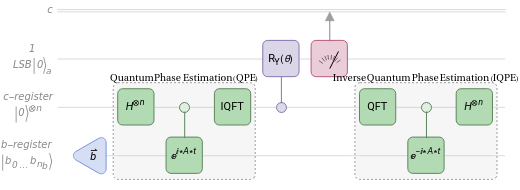
The quantum circuit implementing HHL (as shown in the schematic) is organized into five main sections:
Out[]=
◼
State preparation
b
◼
The vector is encoded into the amplitudes of a register of qubits (the b-register). This step translates the classical problem into a quantum state
b
|b〉.
◼
Quantum Phase Estimation (QPE)
◼
QPE is applied to decompose in the eigenbasis of The eigenvalues of are encoded into an auxiliary register of clock qubits (the c-register).
|b〉
A.
λ
i
A
◼
Controlled Rotation & Measurement of the ancilla qubit
◼
An auxiliary qubit (the ancilla, Least Significant Bit - LSB) is rotated in a way that depends on the eigenvalues stored in the c-register. This step effectively implements the action of , since the amplitudes are scaled by Measure the ancilla and keep only outcomes .
-1
A
1/.
λ
i
|1〉
a
◼
Inverse Quantum Phase Estimation (IQPE)
◼
The inverse QPE is applied to disentangle the c-register from the b-register, ensuring that the solution is properly isolated in the latter.
◼
Measurement
◼
After post-selecting the ancilla in the desired state, the quantum system in the b-register encodes the solution While the algorithm does not yield the classical solution vector directly, it enables the estimation of global properties of the solution, such as norms, probability distributions, or expectation values of observables.
|x〉=|b〉.
-1
A
This way, HHL combines three central tools of quantum computing:
◼
superposition
◼
phase estimation
◼
controlled operations
And turn it into a coherent algorithm that addresses a fundamental problem in science and engineering.
Encoding Scheme
Encoding Scheme
We implement the HHL algorithm for the following system of linear equations:
|
with
A=
,=
1 | -1/3 |
-1/3 | 1 |
b
0 |
1 |
In[]:=
A=1,,,1;b={0,1};
-1
3
-1
3
The eigenvalues and eigenvectors of 𝐴 are:
In[]:=
Eigensystem[A]
Out[]=
,,{{-1,1},{1,1}}
4
3
2
3
In[]:=
{λ1,λ0}=Eigenvalues[A]
Out[]=
,
4
3
2
3
To encode the eigenvalues in the clock register, we use basis encoding. Two qubits are sufficient to represent the eigenvalues while maintaining their ratio:
λ
0
|01〉
λ
1
|10〉
This preserves the ratio /=0:
λ
0
λ
1
In[]:=
n=Divide@@Eigenvalues[A]
Out[]=
2
This gives a perfect encoding with (i.e., ). The evolution time 𝑡 is chosen to satisfy:
𝑛=2
𝑁==4
n
2
λ
j
Nλ
j
In[]:=
Solve1==*λ0*t,{t}
n
2
2π
Out[]=
t
3π
4
In[]:=
Solve2==*λ1*t,{t}
n
2
2π
Out[]=
t
3π
4
Since is a 2-dimensional vector, it can be encoded using one qubit, so =1
b
n
b
The exact solution to the linear system is:
In[]:=
LinearSolve[A,b]
Out[]=
,
3
8
9
8
We can verify the ratio of the squared amplitudes :
:=1:9
x
1
2
x
2
2
In[]:=
Divide@@
2
Reverse[%]
Out[]=
9
Implementation of the controlled-rotation of ancilla qubit
Implementation of the controlled-rotation of ancilla qubit
The next step is to rotate the ancilla qubit using a controlled RY(θ) rotation, where the control comes from the encoded eigenvalues in the clock (c-) register.
|0〉
a
The rotation maps:
|0〉
a
1-
C
2
λ
j
|0〉
a
C
λ
j
|1〉
a
with and C is a constant chosen to maximize the probability of measuring .
θ=2ArcSin
C
λ
j
|1〉
a
The sum of the squares of the coefficients of and is 1, as required for a normalized quantum state. This also implies that for all eigenvalues. Since the minimal =1 in our example, we set to maximize the probability of measuring during the ancilla measurement.
|0〉
|1〉
C<=
λ
j
λ
j
C=1
|1〉
a
To implement this rotation in the algorithm,we solve for θ in terms of the encoded eigenvalues:
In[]:=
rotation=QuantumOperator["RY"[θ]]@QuantumState["0"];rotation["Formula"]
Out[]=
Cos|0〉+Sin|1〉
θ
2
θ
2
In[]:=
θsolutions=Solverotation["AmplitudeList"]==,{θ}/.ArcCos[x_]:>ArcSin
1-
,1
2
λ
1
λ
1-
//FullSimplify//Quiet2
x
Out[]=
θ-2ArcSin,θ2ArcSin
1
2
λ
1
2
λ
Assigning the actual eigenvalues:
In[]:=
θvalues=θ/.Last[θsolutions]/.->{1,2}
λ
Out[]=
π,
π
3
When the ancilla qubit is measured, it collapses to either or :
|0〉
a
|1〉
a
◼
If it collapses to , the computation is discarded and repeated.
|0〉
a
◼
If it collapses to , the resulting state is proportional to the solution , but the b-register is still entangled with the clock register.
|1〉
a
|x〉
To obtain the correct amplitudes in the computational basis, we need to uncompute the clock register. This disentangles the b-register from the clock qubits.
Quantum Phase Estimation
Quantum Phase Estimation
Quantum Phase Estimation (QPE) is a core eigenvalue estimation algorithm used in HHL. It consists of three main steps:
◼
Creating a superposition of the clock qubits using Hadamard gates.
◼
Performing the inverse quantum Fourier transform (IQFT) on the clock register.
For our 2×2 example (𝑛=2), the required operations are:
Inspecting the resulting matrix:
We can also implement QPE directly using the built-in “PhaseEstimation” gate in Wolfram Language:
Note that in our framework, the controlled-unitary gates are constructed in the opposite direction compared to this paper conventions. (remove this, focus only on our convention, we do not want to say we reproduce exactly a specific result etc)
Circuit Implementation
Circuit Implementation
We can now implement the full HHL algorithm as a quantum circuit in Wolfram Language. The circuit includes the following steps:
◼
Apply Quantum Phase Estimation (QPE) on the clock qubits.
◼
Perform controlled RY(θ) rotations on the ancilla qubit, using the angles computed from the encoded eigenvalues.
◼
Uncompute the QPE to disentangle the b-register from the clock qubits.
◼
Measure the b-register to extract the solution.
We can visualize the circuit:
Perform the measurement:
After executing the circuit and measuring the qubits, the probabilities of each computational basis state are:
The solution correspond to the measured probabilities of the b-register. Selecting the relevant outcomes:
Finally, we verify that the ratio of the measured amplitudes matches the ratio of squared solutions obtained classically:
This confirms that the HHL implementation successfully encodes the solution to the linear system in the amplitudes of the b-register, consistent with the classical solution.
Multiplexer-Based Quantum Linear Solver
Multiplexer-Based Quantum Linear Solver
Theory
Theory
The Variational Quantum Linear Solver (VQLS) is a a hybrid quantum-classical technique designed to address the Quantum Linear Systems Problem (QLSP). It aims to find linear system solutions using quantum computing techniques.
The classical problem is formulated as follows:
The corresponding quantum algorithm can be summarized as follows:
Given:
We want to prepare:
Multiplexer-based VQLS
Multiplexer-based VQLS
The primary distinctions between MB–VQLS and a conventional VQLS lie in two key aspects:
◼
Quantum fidelity cost function:
◼
The solution to the linear system is encoded directly in the amplitudes of the resultant quantum state.
Initial problem setup
Initial problem setup
As we previously discussed, we need to save the normalization terms, since we will be working with the normalized matrix and vector:
Multiplexer implementation
Multiplexer implementation
Next, implement the multiplexer:
We obtain the first section of the variational circuit for the VQLS:
Optimization
Optimization
In other words, this cost function does not ensure that the amplitudes of both states are identical, but rather that they are proportional by a global phase:
Implement the cost functions previously defined, rememer to use the normalized vector b:
Now, let’s optimize the cost function using FindMinimum, with our initial guess as the starting point:
As we can see, FindMinimum is having some difficulty finding the minimal value, so we might switch to NMinimize, which will return a value for the cost function that is very close to zero:
As we can notice, the values are quite close! However, as mentioned earlier, while the probability distributions match, the amplitudes do not necessarily align:
We can verify our result: