Quantum Natural Gradient Descent

〈 Back

Gradient-based optimization methods represent a cornerstone in the field of numerical optimization, offering powerful techniques to minimize or maximize objective functions in various domains, ranging from machine learning and deep learning to physics and engineering.

In this lesson we will be talking about optimization. We have always performed optimization during the previous sections using big tools such as NMinimize, FindMinimum, and others.

There are various approaches to performing optimization, but gradient-based methods are particularly useful for accelerating the process and ensuring convergence.

But what exactly are these gradient-based methods? The term refers to optimization techniques that use the gradient (or higher-order derivatives) of the cost function to guide parameter updates toward minimizing the objective function.

Load Quantum Framework

Using Wolfram Quantum Framework

In[]:=

PacletInstall["https://wolfr.am/DevWQCF",ForceVersionInstall->True]

Out[]=

PacletObject

Name: Wolfram/QuantumFramework

Version: 1.6.0



In[]:=

<<Wolfram`QuantumFramework`

Load QuantumOptimization paclet

In[]:=

<<Wolfram`QuantumFramework`QuantumOptimization`

Refer to the Quantum Optimization documentation.

Parameter Shift Rule

Quantum Circuit Derivative?

Now, you might be wondering: how do we compute the derivative of a quantum circuit?

Great question! While it may seem complex at first, the process is actually quite manageable,and, thanks to the Parameter Shift Rule (PSR), it can even be done analytically!

PSR is a mathematical technique that enables the computation of a quantum circuit’s gradient by evaluating the expectation value twice, each time with one parameter shifted by a fixed amount.

The expected value of a circuit in relation to a measurement operator

varies smoothly with the circuit’s gate parameters

Out[]=

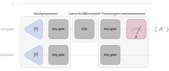
Typically, the quantum circuit whose gradient we seek consists of multiple gates. Here, we’ll focus on computing the gradient for a specific type of unitary gate

U(θ)

Any unitary gate can be cast in the form

iθG

, where

is the Hermitian generator of the gate

. Then let’s assume that every gate before it is the initial state and then every gate after is part of the measurement. Let’s call this expected value of A:

Out[]=

In order to apply the parameter shift rule we need to “shift” our parameter for a given value, you can use pi/2. Then we calculate the difference between the shifted expected values of A:

Out[]=

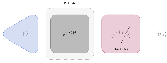
The parameter–shift rule states that in order to obtain the derivative

∇

〈A〉

from gate

, we need to compute:

∇

〈A〉=

Aθ+

-Aθ-



Let’s say that we have this simple circuit with a rotation in x with a measurement in Z:

In[]:=

RXCircuit=QuantumCircuitOperator[{"RX"[θ],QuantumMeasurementOperator["Z"{1,-1}]},"Parameters"->{θ}];RXCircuit[θ]["Diagram",ImageSizeSmall]

Out[]=

If we check the mean value it is:

In[]:=

RXCircuit[θ][]["Mean"]//ComplexExpand//Simplify

Out[]=

Cos[θ]

Applying the parameter shift rule shows that indeed we obtain the derivative:

In[]:=

(RXCircuit[θ+π/2][]["Mean"]-RXCircuit[θ-π/2][]["Mean"])//ComplexExpand//Simplify

Out[]=

-Sin[θ]

The parameter–shift rule only works for gates of the form

θG



where

, in other cases that does not fulfill these conditions, the stochastic parameter–shift rule must be used.

The main benefit of Parameter Shift Rule is that it enables the use of the Gradient Descent optimizer for variational circuits.

Stochastic Parameter Shift–Rule

The Stochastic Parameter Shift Rule (SPSR) represents a powerful optimization technique specifically tailored for parameterized quantum circuits.

Unlike conventional gradient-based methods, SPSR offers a stochastic approach to computing gradients, making it particularly well-suited for scenarios involving noisy quantum devices or large-scale quantum circuits. At its core, SPSR leverages the principles of quantum calculus to estimate gradients by probabilistically sampling from parameter space and evaluating the quantum circuit’s expectation values.

By incorporating random perturbations in parameter values and exploiting symmetry properties, SPSR effectively mitigates the detrimental effects of noise and provides robust optimization solutions.

If G is the generator of the gate U we are about to differentiate, we first express

as a sum of tensor product of Pauli operators

G=H+θV

, where

is a tensor product of Pauli operators and H represents any linear combination of tensor products involving Pauli operators, chosen arbitrarily.

The SPSR algorithm require us to implement the following 3 gates:

Out[]=

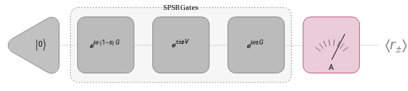
where s is a uniform random variable in the interval

[0,1]

, which we will be sampling multiple times for each θ. The expected value of this circuit will be called

〈

〉

〈

〉

depending on the ϕ shift sign. The gradient can be obtained from the average:

∇

〈A〉=

sϵ[0,1]

[〈

〉-〈

〉]

Example on a Cross–Resonance gate

The cross–resonance gate is be defined as:

(

)=exp[(

X-

ZX+

X)]

Implement the correspondent generator and gate:

In[]:=

CrossResonanceGenerator=QuantumOperator[(θ1*QuantumOperator[{"X"->{1},"I"->{2}}]-θ2*QuantumOperator[{"Z"->{1},"X"->{2}}]+θ3*QuantumOperator[{"I"->{1},"X"->{2}}]),"Parameters"->{θ1,θ2,θ3}];

In[]:=

CrossResonanceGate=QuantumCircuitOperator[{Exp[I*CrossResonanceGenerator],QuantumMeasurementOperator["PauliZ"->{1,-1}]},"Parameters"->{θ1,θ2,θ3}];

In[]:=

CrossResonanceGate["Diagram"]

Out[]=

Let’s calculate our circuit’s gradient for θ ϵ [0 , 2π] using 10 s–random values. First implement the required inputs:

Lets also calculate the mean value too:

We can check the values in a plot and notice that both look like sinusoidal functions:

We can verify our suspicion finding analytical solutions using Fourier interpolation:

The Approximate Stochastic Parameter-Shift Rule

In contrast with the regular SPSR we got some extra terms ϵ and H in the sandwiched gate:

Example on a Cross–Resonance Gate

The implementation of a single ASPSR circuit would be the following:

First we need to implement the H operator from our generator:

Now we can define the circuit:

Since the calculation is basically the same compared to the standard SPSR algorith, we will directly use the function ASPSRGradientValues to compute the gradient, which needs the same input than the SPSR version but including the H operator:

Lets plot it along with the previous result:

We can verify their match using Fourier interpolation:

Gradient Descent

From an analytical perspective, setting the gradient equal to zero and solving for the parameters would give us the solution. However, this is not something a computer can easily compute. Instead, computers rely on calculating the gradient to “move toward the minimum.”

One optimizer that stands out in this context is the well-known Gradient Descent!

Gradient Descent is a fundamental optimization technique used to minimize a function. It is widely used across various fields, such as machine learning, numerical optimization, and quantum computing.

The goal of Gradient Descent is to find the minimum of a cost function by adjusting the parameters iteratively in the direction of the steepest descent of the function being minimized as you can see in this image equation:

◼

Initialization

◼

Begin with an initial set of parameters. This initial guess can either be random or from a heuristic approach.

◼

Update parameters

◼

Adjust the parameters in the opposite direction of the gradient to minimize the function. The update rule is the one in the image.

◼

The learning rate, is a small positive scalar that controls the step size towards the minimum.

◼

Iterate Until Convergence

◼

Repeat steps 2 and 3 until a stopping criterion is satisfied.

This criterion could be based on a threshold for changes in the function value or when the gradient’s magnitude falls below a specific limit, indicating that further updates won’t substantially improve the result. In some cases, steps 2 and 3 may simply be performed for a fixed number of iterations.

Also, selecting an appropriate learning rate is critical: if it’s too small, convergence will be slow; if it’s too large, it can lead to oscillations or even divergence.

VQE Example

So in this case we can calculate a symbolic minimum value of the function using MinValue:

In order to visualize the optimization process, we need to get all the parameter values during the evolution. In this case, we will use the gradient descent method:

Define an initial position:

Use GradientDescent by using the cost function and the initial position as input:

In this case the "LearningRate" and "MaxIteration" are options and we used the default values.

Check the Cost Curve or Loss Curve:

Here we can see that the cost function value is getting lower gradually in each step until converging into the minimum value in only 4 steps!

Remember last class we saw a ContourPlot with higher and lower values? Now we can visualize how the optimization navigates thought the parameter space:

This is consistent with the symbolic gradient!

Let’s analyze the impact of the learning rate η, by default η is 0.8 but we can fix it now to 0.1 :

As you can see, lowering the learning rate made the optimization take more steps!

This can be a little tricky, depending on the parameter space you need bigger or smaller learning rate in order to converge faster to the solution, is not always bigger steps the better option!

Now, we could compare how the paths are different in the parameter space:

In this ContourPlot, the white line is the new path we created using learning rate 0.1. This is pretty interesting to observe because one would imagine that they could follow the same path but skipping steps, but that’s not the reality.

We obtained a pretty smooth curve that by looking at it seems that it is going step by step with the contours, while the original optimization with 0.8 of learning rate go straight to do the work skipping all the possible values and reaching the solution.

Quantum Natural Gradient Descent

Natural gradient descent

When working with the gradient descent, we assume a flat or euclidean parameter space. The algorithm won’t take in account the geometry intrinsic to the cost function which would lead to an inefficient search of the minimal value, as we can see in the step definition, it only depends on the direction of the negative gradient and the learning rate eta.

Fubini–Study metric tensor

So what happens when we have a quantum optimization problem? When using a Quantum Variational Algorithm, we will face a similar problem. In this case the parameter space is defined in the space of quantum states.

In order to understand this, we should think about “distance” in the quantum state:

◼

Definition for distance:

◼

The distance between any two points is always greater than or equal to zero. Furthermore, the distance between two points is zero if and only if those two points are the same.

◼

The distance between two points is the same regardless of the order in which we measure them. That is, the distance from x to y is equal to the distance from y to x.

◼

The distance between two points x and z must be less than or equal to the sum of the distances from x to y and from y to z

The first property is key for defining a correct distance function for quantum states.

◼

Extra physical condition:

This means that the distance will be defined in a projective Hilbert space. A projective space is obtained from a vector space by identifying vectors that differ by a nonzero factor. We need a differential form that does not distinguish parallel vectors ( this means that we are looking for a metric in projective space, which includes non-normalized states).

which defines the component of the differential of psi orthogonal to the state psi. This equation becomes easier to understand when you refer to the vectors in the image:

Aiming to get rid of the “information” from the state projections:.

From normalizing this expression, the norm of this “measurement of changes in the projective space” gives the differential form of the distance which is the Fubini-Study metric:

With this concept in mind, we can now understand how the formula for the Fubini-Study metric is derived. For further exploration of the theory, you can refer to literature on the Quantum Geometric Tensor.

Implement a simple single qubit state:

Let’s calculate the ket, bra and cost function by applying the VQE over a single Pauli X hamiltonian:

Apply the FubiniStudyMetricTensor function to obtain the calculated QuantumOperator:

The Fubini-Study metric tensor plays a crucial role in Quantum Natural Gradient Descent. Originating from the field of differential geometry, the Fubini-Study metric tensor enables the quantification of distances between quantum states on the complex projective Hilbert space.

Quantum Natural Gradient Descent

In the context of Quantum Natural Gradient Descent, the Fubini–Study metric tensor serves as a fundamental tool for characterizing the geometry of the parameter space associated with parameterized quantum circuits. The update rule is the following:

By incorporating the Fubini-Study metric tensor into the optimization process, this algorithm effectively accounts for the curvature of the quantum state manifold, enabling more precise and efficient updates of circuit parameters.

Let’s compare the optimization process:

First, we define a function for the cost function from the previous example:

Next, we apply the QuantumNaturalGradientDescent function using energy and the Fubini-Study metric tensor we calculated, with the initial point and learning rate set as follows:

At the same time, we compare this with regular Gradient Descent and evaluate the results:

As expected, the Quantum Natural Gradient Descent optimization reaches the ground state before the regular Gradient Descent, as shown in the plot:

This degeneracy also corresponds to a singularity in the natural gradient:

We can observe this behavior in the optimization’s evolution, as shown in the contour plot. In this plot, regular gradient descent passes directly through the singularity, eventually finding a minimum, while Quantum Natural Gradient Descent appears to avoid the singularity and finds a different minimum value.:

Block-diagional approximation

The circuit is given by:

The quantum state before the application of layer l is:

Let’s build a circuit for the following example:

Exact Fubini-Study metric tensor

First, we will implement the exact metric tensor based on our current formulation:

Test with the following initial parameters:

Block-diagional metric tensor approximation

sing the block-diagonal approximation, we will try to match the earlier result.

In this case we got 2 parametrized layers with two parameters each, then following the block-diagonal approach:

Let’s define some helping functions:

Calculate the first layer using the following formula:

The second layer:

Then the block diagonal matrix is the following:

Cost function

Optimization

The ground state is reached in less steps by the quantum gradient descent.