Quantum Approximate Optimization Algorithm

〈 Back

The Quantum Approximate Optimization Algorithm (QAOA) is a well-studied approach for solving combinatorial optimization problems.

Theory

Combinational Optimization

The combinatorial optimization problem involves finding an optimal object from a finite set of objects. This problem can be formulated as maximizing an objective function, which is expressed as a sum of Boolean functions.

Each Boolean function

{0,1}

->{0,1}

takes a n-bit string

…z

as input and produces a single bit (0 or 1) as output.

For a problem with n bits and m clauses, the goal is to find a n-bit string z that maximizes the function:

C(z)=

∑

i=1

(z)

Approximate optimization aims to find a near-optimal solution to this problem, which is often NP-hard. The approximate solution is an n-bit string z that closely maximizes the objective function 𝐶(z).

Quantum Approximate Optimization Algorithm

The Quantum Approximate Optimization Algorithm (QAOA) is a well-studied approach for solving combinatorial optimization problems. First proposed by Edward Farhi as a Variational Quantum Algorithm (VQA) designed to find approximate solutions to the Max–Cut problem, and to be executable on Near–term Intermediate–Scale Quantum (NISQ) devices.

The QAOA was formulated as a variational approach that alternates between cost and mixer layers. Specifically, QAOA applies a sequence of alternating unitaries: the cost unitary

(

)

and the mixer unitary

(

)

, where

denotes the layer index. The central idea is to encode the objective function of a combinatorial optimization problem into a cost Hamiltonian

, and then variationally optimize the parameters to search for an optimal bitstring.

The QAOA process involves the following steps:

◼

Defining a Cost Hamiltonian

This Hamiltonian is designed such that its ground state encodes the optimal solution to the combinatorial optimization problem.

◼

Defining a Mixer Hamiltonian

This Hamiltonian is used to explore the solution space by driving transitions between different states.

◼

Defining the unitary gates:

(γ)=

-*\bt*

(γ)



(θ)=

-*\bθ*

(θ)



◼

Applying the gates alternately in layers, forming the unitary:

U(γ,θ)=

∏

i=1

(γ)

(θ)

◼

Preparing an Initial State and Applying

U(t,θ):

The initial state is typically a superposition of all possible states. The alternating application of

and

evolves this state according to the chosen parameters.

◼

Optimizing Parameters and Measuring:
Classical optimization techniques are used to adjust the parameters t and θ to maximize the expectation value of the cost Hamiltonian

The measurement of the final state provides an approximate solution to the original problem.

Max-Cut Problem

The Max–Cut problem is one of the most prominent and widely studied combinatorial optimization problems. It consists of finding a partition of the vertices of a graph into two complementary subsets in such a way that the total weight of the edges crossed by the cut is maximized.

Formulating Max-Cut with Classical Binary Variables

Consider an undirected graph

G=(V,E)

, where V is the set of vertices, E the set of edges, and

denotes the weight of the edge

(i,j)∈E

, connecting vertices

and

. The goal is to partition the graph vertices

for

iϵ{1,…,V}

, into two complementary subsets labeled as

∈{-1,1}

in such a way that the total weight of the edges between vertices in different subsets is maximized.

In[]:=

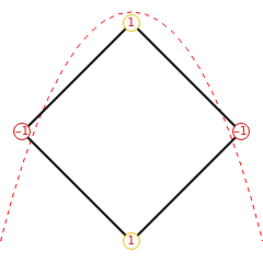
g=GraphRange[4],UndirectedEdge@@@{{1,2},{1,4},{2,3},{3,4}},

;highlited=HighlightGraphg,(Subgraph[g,#]&)/@Last[FindMaximumCut[g]],



;cut=Show

Graphics[

]

,highlited,

;GraphicsRow[{g,cut}]

Out[]=

Considering the plain Max-Cut problem



=1

, this sumation is defined as:

∑

,∈V

1-





,s∈{-1,+1}

Analyzing the following cost function, we notice:

◼

and

have opposite signs:The cut contributes to the objective function because the vertices are placed in different sets. Mathematically, this happens because

=1-





◼

and

have same sign:Then they remain in the same subset, meaning there is no cut and the edge does not contribute to the objective function because

=1-





Use the Wolfram Language function FindMaximumCut to solve the classical Max-Cut problem:

In[]:=

FindMaximumCut[g]

Out[]=

{4,{{1,3},{2,4}}}

This follows the solution given in the first image:

In[]:=

cut

Out[]=

Formulating Max-Cut with Quantum Mechanics

To solve the Max-Cut problem on a quantum computer, we need to reformulate it in terms of quantum mechanics. Specifically, we convert the classical optimization problem into one of finding the eigenstate of a quantum Hamiltonian.

In the classical case, we represent a solution using a binary string where each

vertex

has an associated value



∈{-1,1}

. In the quantum case, we represent each vertex using a qubit. Since the eigenvalues of Z are also ±1, we map these classical binary variables onto the eigenvalues of the Pauli-Z operator.

Our goal now shifts from finding a binary string to identifying the highest-energy eigenstate of a quantum Hamiltonian.

◼

To proceed, we first load the Wolfram Quantum Framework:

In[]:=

<<Wolfram`QuantumFramework`

In[]:=

<<Wolfram`QuantumFramework`QuantumOptimization`

Hamiltonian formulation

Max-Cut Hamiltonian obtained by mapping the binary variables

onto Pauli-Z eigenvalues:

∑

,∈V

-







where the

operator acts on the

i-th

qubit (node).

Represent each node as a qubit, then we have the bitstring:

…x

〉

By applying the

operators to the bitstring, we can gain insight into its behavior, which is useful for reformulating the problem:

…x

〉=

(-1)

…x

〉,

∈{0,1}

Based on this result, we switch from the classical variables

∈{-1,1}

∈{0,1}

, in order to label the two complementary subsets being cut.

Considering the initial problem, we can implement

using the Graph functionalities:

In[]:=

index=MapApply[List,EdgeRules[g]]/.x_Integer:>{x,x};op=StringRepeat["I",VertexCount[g]];sum=Total

(op-StringReplacePart[op,"Z",#])&/@index

Out[]=

IIII-IIZZ

IIII-IZZI

IIII-ZIIZ

IIII-ZZII

We’ve defined the summation and specified which qubits are coupled via

operators. You can also write the Pauli operators manually as an String.

Next, we generate the Cost Hamiltonian QuantumOperator:

In[]:=

Hc=QuantumOperator[sum]

Out[]=

QuantumOperator

Pure map
Dimension: 16→16	Order: {1,2,3,4}→{1,2,3,4}



Solution analysis


Understanding QAOA Ansatz

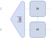
To implement the Max-Cut problem on a quantum computer, we start by putting the nodes in superposition. This ensures that each node (qubit) has an equal probability of being in either partition.

In[]:=

superposition=QuantumCircuitOperator[{"00","HH"},"Label"->"

4

|+〉

"];superposition["Diagram",ImageSizeSmall]

Out[]=

Some initial intuition comes from our first example, which involves identifying a periodic pattern, such as 0101 or 1010, within a bitstring.

To achieve this, we need to establish connections between nodes or qubits that reflect the structure of the cost Hamiltonian. For this initial idea, we can evaluate the gate sequence CNOT + RZ + CNOT.

We can verify that it distinguish the possible correct solutions from the non-periodic bitstrings in order to solve the problem:

We can gain some initial insights and visualize the differences in the solution amplitudes in the following plot:

The concept becomes clearer when we observe that the probabilities of regular bitstrings are minimal when the probabilities of periodic bitstrings are maximal, and vice versa:

The set of gates outlined earlier is commonly referred to as an RZZ gate, which combines rotations and controlled operations:

Now that we understand this, we can apply it to every pair of qubits connected in the graph. In other words, we apply the RZZ gate to every edge in the graph. This ensures that the quantum state evolves according to the problem constraints.

The previous step does not explore all possible cuts because some amplitudes remain unchanged, so we need to mix things a little bit!

Visualize the symbolic function corresponding to each possible state:

Considering the initial state preparation, we recover a mini-QAOA:

The increased expressibility of the resulting state from this ansatz, as compared to previous circuits, comes from the final mixing performed by the mixing layer of gates:

From the following plot, we can observe how the probabilities for regular and periodic bitstrings oscillate, similar to the previous plots. The new parameter θ does not interfere with this behavior; instead, it expands the parameter space, providing additional expressibility to our ansatz:

Step–by–Step: 4-Edge Graph Example

Find the Max-Cut for the following graph:

Implement the Cost Hamiltonian:

Initial state preparation for superposition:

We can use Wolfram Mathematica's Graph functionalities to establish connections between qubits within the Cost-Circuit:

This layer of gates actually corresponds to the operator generated by the Cost Hamiltonian we defined earlier:

To ensure full exploration, we need a mixer Hamiltonian that allows transitions between different states:

Define the variational states to calculate the Cost function:

Let's try out the NMaximize optimizer:

We can enhance the precision of our solution by increasing the number of QAOA layers. This is easy to do since we can use QuantumCircuitOperator with the previous circuit but replacing the parameters:

We can utilize the Parameters option from the Wolfram Quantum Framework to re-name the gate parameters, allowing us to distinguish one layer from another.

Implement the cost function:

Optimimize:

Now, we obtain the exact result.

This solution represents the cut shown in the first image of this section:

Example: 5-Edge Graph

With a clear understanding of each step involved in solving the Max-Cut problem using QAOA, we are now ready to proceed with the direct implementation of the solution.

Find the Max-Cut for the following graph:

In this more challenging example, we will generate the Hamiltonian programmatically instead of writing it explicitly:

Implement directly the QAOA circuit using the Graph functionalities:

Implement the symbolic cost function using the Cost Hamiltonian and the resulting parametrized state from the previous circuit:

Use NMaximize for the optimization:

We obtain multiple possible solutions; however, with just a single QAOA layer, we observe four solutions with higher probability:

Solve it clasically:

The quantum algorithm does not achieve the maximum value compared to the classical solution, but we can analyze the four most probable solutions indicated by the ProbabilityPlot:

Example: 6-Edge Graph

Find the Max-Cut for the following graph:

In this more challenging example, we have a graph with six nodes, which results in a much larger cost Hamiltonian:

Implement directly the QAOA circuit using the Graph functionalities:

Implement the symbolic cost function using the Cost Hamiltonian and the resulting parametrized state from the previous circuit:

Use NMaximize for the optimization:

We obtain multiple possible solutions; however, with just a single QAOA layer, we observe four solutions with higher probability:

Solve it clasically:

The quantum algorithm does not achieve the maximum value compared to the classical solution, but we can analyze the four most probable solutions indicated by the ProbabilityPlot:

QAOA-in-QAOA for Maxcut

To tackle large graphs, we use a method called QAOA-in-QAOA, inspired by the Divide and Conquer algorithm.

Here’s the idea:

◼

First, we partition the graph into smaller subgraphs.

◼

Next, we solve a mini-QAOA on each subgraph and combine the solutions.

◼

Then, to correct any possible issue with the solutions between the subgraphs, we treat each subgraph as a node in a new coarse-grained graph.

◼

Finally, we apply QAOA again to this higher-level graph and correct the final solution.

This process is recursive and scalable, making it suitable for large problem instances.

Now let’s see how the Wolfram Quantum Framework enables us to symbolically model and analyze this algorithm. Given the following graph:

Given the following partition:

Divide (Subgraphs)

We load the Hamiltonian for each minigraph:

We then construct symbolic QAOA circuits, with qubit indices mapping directly to graph nodes:

After simulating the states, we can observe how the symbolic computation can give insights about cost functions for each subgraph. We can visualize the parameter space using contour plots, giving us deep insight into the optimization behavior.

After just a single QAOA layer, we already discover useful solutions:

Each minigraph contributes to a partial solution, illustrated by colored nodes yellow and red:

Conquer (Big graph)

In the Conquer phase, we construct a new graph where each node represents a subgraph, and the edges are based on their prior connections:

We then assign weights based on inter-subgraph interactions and repeat the QAOA process at this higher level:

Finally, we observe the resulting probability distribution and solve the MaxCut problem for the higher-level graph:

In the final step, we take the subgraphs that are yellow nodes in the higher level graph and flip their node values. For instance, in some subgraphs, yellow nodes may become red, as the global optimization balances local and global constraints.

Quantum Approximate Optimization Algorithm

Theory

Combinational Optimization

Quantum Approximate Optimization Algorithm

Max-Cut Problem

Formulating Max-Cut with Classical Binary Variables

Formulating Max-Cut with Quantum Mechanics

Hamiltonian formulation

Solution analysis

Understanding QAOA Ansatz

Step–by–Step: 4-Edge Graph Example

Example: 5-Edge Graph

Example: 6-Edge Graph

QAOA-in-QAOA for Maxcut

Divide (Subgraphs)

Conquer (Big graph)

Solution analysis
