Vostok - Revision of the EPICA Dome C CO2 record from 800 to 600 kyr BPCO2 Frequencies estimatesNOAA Paleoclimatology ProgramNational Centers for Environmental Information (NCEI)(fully coded)
Dara O Shayda
dara@compclassnotes.com
dara@compclassnotes.com
In[]:=
DateObject[]
Out[]=
Abstract
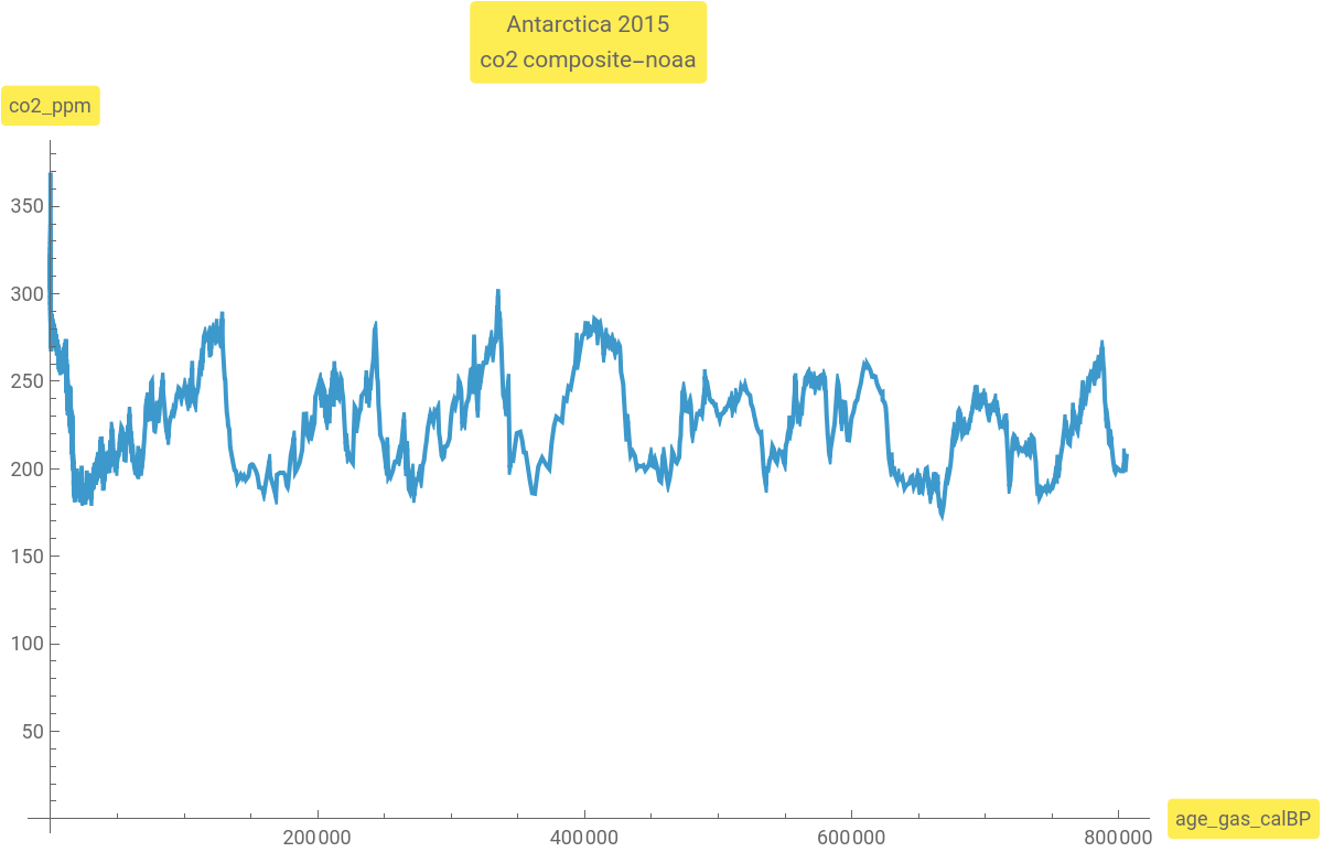
This live code notebook acquires the revised data from the European Project for Ice Coring in Antarctica Dome ice core from Dome C (EDC) has allowed for the reconstruction of atmospheric CO2 concentrations for the last 800,000 years [1]. And exclusively computes the CO2 Wavelet decomposition frequencies. A great amount of care and detailed code and advanced 2D and 3D visualizations are gone into the Wavelet Scalograms and the computation of the frequencies for the Vostok CO2 data. And to offer a chance for the public to conduct their own future competent examinations on the impacts of the CO2 on the planet’s climate.

© 2012-Present CCN StudiosCreative Commons Attribution-NonCommercial-ShareAlike 4.0

In[]:=
url="https://www.ncei.noaa.gov/pub/data/paleo/icecore/antarctica/antarctica2015co2composite-noaa.txt";datavos0=Import[url,"Table"];data=ToExpression@Drop[datavos0,143];
In[]:=
datavos0[[143]]
Out[]=
{age_gas_calBP,co2_ppm,co2_1s_ppm}
In[]:=
data[[1]]
Out[]=
{-51.03,368.02,0.06}
In[]:=
ListLinePlot[data[[All,{1,2}]],ImageSize->600,AxesLabel->{Highlighted@"age_gas_calBP",Highlighted@"co2_ppm"},PlotLabel->Highlighted@"Antarctica 2015\nco2 composite-noaa"]
Out[]=
ContinuousWaveletTransform [ ]
● The continuous wavelet transform of a function is given by. ● The continuous wavelet transform of a uniformly sampled sequence is given by .● The scaling parameter is given by equal-tempered scale =α where is the octave number, the voice number, and the smallest wavelet scale.● For each scale , the []computes the wavelet coefficients .
x(t)
w(u,s)=x(t)t
1
s
∞
∫
-∞
*
ψ
t-u
s
{,,…}={x(),x(Δ+),…}
x
1
x
2
t
0
t
0
w(u,s)=
1
s
n
∑
k=1
x
k
*
ψ
Δ(k-u)
s
s
s
oct,voc
oct-1
2
voc/nvoc
2
oct
voc
α
s
oct,voc
ContinuousWaveletTransform
{w(1,),w(2,),…,w(n,)}
s
oct,voc
s
oct,voc
s
oct,voc
In[]:=
cwd=ContinuousWaveletTransform[data[[All,2]],DGaussianWavelet[8],12,SampleRate->Length[data[[All,1]]]]
Out[]=
ContinuousWaveletData


In[]:=
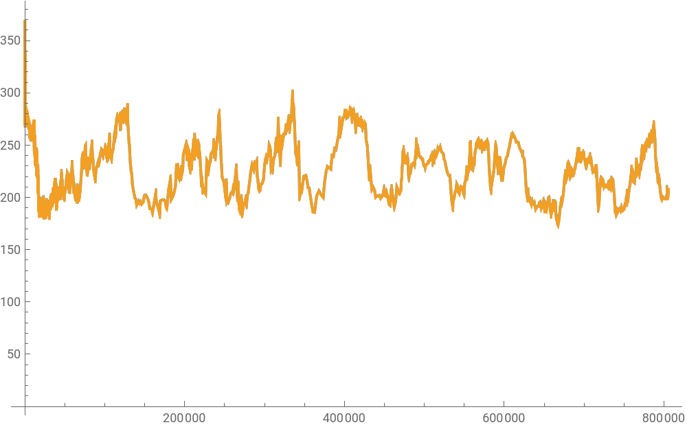
ListLinePlot[{Thread[{data[[All,1]],data[[All,2]]}],Thread[{data[[All,1]],InverseContinuousWaveletTransform[cwd]}]},ImageSize->500,PlotLegends->{"Original","Inverse"}]
Out[]=


In[]:=
cwd["IndexMap"]
Out[]=
{{1,1},{1,2},{1,3},{1,4},{2,1},{2,2},{2,3},{2,4},{3,1},{3,2},{3,3},{3,4},{4,1},{4,2},{4,3},{4,4},{5,1},{5,2},{5,3},{5,4},{6,1},{6,2},{6,3},{6,4},{7,1},{7,2},{7,3},{7,4},{8,1},{8,2},{8,3},{8,4},{9,1},{9,2},{9,3},{9,4},{10,1},{10,2},{10,3},{10,4},{11,1},{11,2},{11,3},{11,4},{12,1},{12,2},{12,3},{12,4}}
In[]:=
cwd["Properties"]
Out[]=
{DataChannels,DataDimensions,DataMean,DataWrapper,LinearScalogramFunction,ListPlot,LogScalogramFunction,Octaves,Properties,SampleRate,Scales,Voices,Wavelet,WaveletIndex,WaveletScale}
In[]:=
cwd["Octaves"]
Out[]=
12
There is an inverse relationship between scale values and frequency values:
In[]:=
freq=#11&/@cwd["Scales"]
cwd["SampleRate"]
#1〚2〛
Out[]=
{{1,1}3445.05,{1,2}2896.93,{1,3}2436.02,{1,4}2048.44,{2,1}1722.52,{2,2}1448.46,{2,3}1218.01,{2,4}1024.22,{3,1}861.261,{3,2}724.232,{3,3}609.004,{3,4}512.109,{4,1}430.631,{4,2}362.116,{4,3}304.502,{4,4}256.055,{5,1}215.315,{5,2}181.058,{5,3}152.251,{5,4}128.027,{6,1}107.658,{6,2}90.529,{6,3}76.1255,{6,4}64.0136,{7,1}53.8288,{7,2}45.2645,{7,3}38.0627,{7,4}32.0068,{8,1}26.9144,{8,2}22.6322,{8,3}19.0314,{8,4}16.0034,{9,1}13.4572,{9,2}11.3161,{9,3}9.51569,{9,4}8.00171,{10,1}6.72861,{10,2}5.65806,{10,3}4.75784,{10,4}4.00085,{11,1}3.3643,{11,2}2.82903,{11,3}2.37892,{11,4}2.00043,{12,1}1.68215,{12,2}1.41452,{12,3}1.18946,{12,4}1.00021}
Match Frequency Range to Refinements
In[]:=
Cases[freq,u_/;(2048.436599092417`≤Last[u]≤3445.0459861026484`)]
Out[]=
{{1,1}3445.05,{1,2}2896.93,{1,3}2436.02,{1,4}2048.44}
Digression: Colorization of Scalogram and what colors mean
Create a single with two periodic additive components e.g. Cos[20 π x]+Sin[150 π x] .Sample this signal/data at intervals or 1023 sample rate.
1
1023
In[]:=
data2=TableCos[20πx]+Sin[250πx],x,0,1,;ListLinePlot[data2,PlotStyle->Thickness[0.003],ImageSize->500]
1
1023
Now user the ContinuousWaveletTransform[] to compute the signal/data decomposition. As you can see two bands, each fro
Find the Refinements containing the interval [10, 75]
Notice the darker frequency band for refinement {7,2}11.6761 is the lower band or the Trend, somehow the addition of the two carries more of the lower frequency post addition:
Find the Refinements containing the interval [10, 75]
Notice the darker frequency band for refinement {3,4}132.1 is the higher band more towards the Noise, somehow the addition of the two carries more of the Noise frequency post addition due to the larger amplitude 10*Sin[250π x] :
Back to Vostok CO2
Let us plot the decompositions and study their bands. However as you can see the image becomes to blurry:
Live a Little!
Let us get really bold something new here:
1. Extract the image of the scalogram
2. Sharpen 80 times!
3. Apply a RidgeFilter[ ] to expose its venation (ridges) as a mask
5. Image multiply the mask with the Sharpened image of #2
1. Extract the image of the scalogram
2. Sharpen 80 times!
3. Apply a RidgeFilter[ ] to expose its venation (ridges) as a mask
5. Image multiply the mask with the Sharpened image of #2
Less detailed Scalogram with focus on the lower frequency decompositions:
3D Scalogram!
This is a zoomed shot of the 3445.05 frequency top regions of the Scalogram. You can appreciate the frequency landscapes like actual natural landscapes.
3D List Stacked Decompositions!
References
[1] Authors: Bereiter, B., S. Eggleston, J. Schmitt, C. Nehrbass-Ahles, T. F. Stocker, H. Fischer, S. Kipfstuhl, J. Chappellaz
Journal_Name: Geophysical Research Letters
Published_Title: Revision of the EPICA Dome C CO2 record from 800 to 600 kyr before present
Published_Date_or_Year: 2015
Volume: 42
Pages: 542-549
Issue: 2
Report_Number:
DOI: 10.1002/2014GL061957
Journal_Name: Geophysical Research Letters
Published_Title: Revision of the EPICA Dome C CO2 record from 800 to 600 kyr before present
Published_Date_or_Year: 2015
Volume: 42
Pages: 542-549
Issue: 2
Report_Number:
DOI: 10.1002/2014GL061957