OCEAN COLOR Calculus Image IntegrationNASA MODIS-Aqua Satellite(fully coded)
Part 2-α9.0
Dara O Shayda
dara@compclassnotes.com
dara@compclassnotes.com
In[]:=
DateObject[]
Out[]=
Abstract
NASA’s Ocean Color satellites monoidal language is extended with multivariable integration and image segmentation. The image segmentation allows for integration over non-rectangular regions of interest in the satellite images. A Content Addressable Memory system is now included in the monoid to reduce the usage of the assignment operator = . The satellite images are used as addresses to index the monoid’s return values as well as interim computed variables; the storage and ease of access to the interim variables reduce the overly verbose coding as seen in other image processing applications.The monoidal language is an excellent training and teaching tool for calculus and even functional analysis starting from STEM students to graduate students. Note: More of these live notebooks will be released for a variety of variables and ocean regions, notebooks become too large and therefore each variable requires a notebook of its own.
ceanolors[]
ceanolors[]

Software
Release: α9.0 .
Scripts: Symbolic computations performed in Wolfram Mathematica 14.3 .Notebook: https://www.wolframcloud.com/obj/ccn2/Published/ocean_colors_integrals_part2.nb Support: Contact the author for additional code, bugs, correction in maths and algebraic/mathematical mistakes or invalid inferences.Nomenclature: Most functions and most identifiers start with lower case letters, all native vendor identifiers start with upper case. No Packaging: There is no software engineering applied to the code here nor elsewhere in the author’s technical notes to reduce the difficulties and version mismatches in future. The eager readers can simply copy paste the code or download and run the notebook. TODO: 0. Urgently require the color map peer-review to make sure it matches NASA’s satellite instruments documentation. 1. Full JSON ASCII output support for third party Python, JS, C/C++/C# programs.2. Image derivatives are taken on the gray level version of the image, in case the derivatives ought to be taken for each channel.3. One or several Cloud Objects containing the file, its monoids and parametrizations with API Functions for external interactions.This is critical and urgent to allow for large number of variables and scans while the size of the live code notebook would remain small. 4. Login, authorization and Hash for time-stamping and copyrights. 5. Interim images and other related data and computations saved into cloud objects.6. Integration over an image ✓ 7. PDE solutions over one image and over a family of images.8. Wavelets9. Volumetric or 3D image versions and animation flip-books TOLEARN:1. Color maps that match the coloration of the ocean waters as seen by the satellites ✓ 2. Animate regions of oceans in Mathematica, Unity and Blender. Known Issues:1. A rule delayed ParametricPlot3D[ ] might not render with no errors. Running it twice all is normal. This case occurs when plotting the spline images.
© 2012-Present CCN StudiosCreative Commons Attribution-NonCommercial-ShareAlike 4.0

A Quick Computing Tour
● Ocean color is the apparent hue, shade, or tone of water that results from the interactions of sunlight with the microscopic composition of the water column and water itself. Typical relevant water constituents include phytoplankton, mineral particles, and dissolved organic matter. The color of the ocean varies with how these materials in seawater absorb and scatter photons of different wavelengths, which varies with their composition. For example, highly productive waters where phytoplankton are abundant can appear green, whereas less productive waters with fewer constituents typically appear blue.[4]
The spectral nature of color of the water—that is, the intensity at which different wavelengths absorb and scatter photons—can be used to infer the quality and quantity of materials that comprise natural waters, allowing scientists, policymakers, and society as a whole to understand their composition on local to global scales. This understanding can lend insight into how aquatic organisms at the base of the food chain thrive or decline under changing conditions of their environments.
The spectral nature of color of the water—that is, the intensity at which different wavelengths absorb and scatter photons—can be used to infer the quality and quantity of materials that comprise natural waters, allowing scientists, policymakers, and society as a whole to understand their composition on local to global scales. This understanding can lend insight into how aquatic organisms at the base of the food chain thrive or decline under changing conditions of their environments.
● NASA’s Ocean Color satellites systems photograph large swathes of ocean surfaces to record the quantities of these planetary surface waters variables [3], all papers for the calculations of these algorithms included in [3] :
● The concentration of the photosynthetic pigment chlorophyll a
● The diffuse attenuation coefficient for down-welling irradiance over the first optical attenuation layer
● Spectral marine absorption and backscattering coefficients of water column constituents
● PAR at the ocean surface at the time of the satellite observation
● Relative measure of water-leaving radiance associated with chlorophyll fluorescence
● The concentration of particulate organic carbon
● The concentration of particulate inorganic carbon
● Daily mean photosynthetically available radiation at the ocean surface
● The at-surface spectral remote-sensing reflectances observed by the satellite instrument after atmospheric correction. The aerosol optical thickness and aerosol Ångström exponent products are also described.
● Sea surface temperature derived from long-wave (11-12 µm) thermal radiation
● Sea surface temperature derived from short-wave (3-4 µm) thermal radiation
● Sea surface temperature returned in three mid- and long-wave infrared bands
Provisional (proposed)
● Aerosol correction for sea surface temperature
● This algorithm returns the weighted harmonic mean of the visible-range (400 – 700 nm) remote sensing reflectance (Rrs) wavelengths, outputting the Apparent Visible Wavelength (AVW) in units of nanometers.
● This product provides the cloud optical depth (COD) and cloud effective radius (CER).
● The thermodynamic phase of a cloudy pixel: liquid water, or ice crystals.
● The cloud top pressure (CTP) and cloud top height (CTH) for cloudy pixels.
● This algorithm returns the concentration of the phytoplankton carbon.
● This algorithm returns near-surface concentrations of three different phytoplankton groups (cells mL-1): Prochlorococcus, Synechococcus, and autotrophic picoeukaryotes.
● This algorithm derives the concentration of particulate inorganic carbon (PIC) in mol m-3, calculated using an empirical relationship derived from in situ measurements of PIC and remote sensing reflectance (Rrs) in the green-to-red region of the visible spectrum.
● This algorithm returns the Quality Water Index Polynomial (QWIP) score, representing a quantitative metric to evaluate the quality of ocean color remote sensing reflectance (Rrs) data (Dierssen et al. 2022).
● The RemoTAP algorithm determines the quantity, size, and other information about aerosols from images gathered by the SPEXone camera on the NASA PACE satellite.
● Sea surface temperature using a physical deterministic method
● Spectral marine absorption and backscattering coefficients of water column constituents
● Spectral marine absorption and backscattering coefficients of water column constituents
● Depth of the euphotic zone
● The time series of vegetation indices using hyperspectral data from the OCI, and new narrowband indices for leaf pigment content.
● The SFREFL product provides spectrally resolved land surface reflectance.
What is Image Calculus and why bother?
● Any image can easily be parameterized in two variables along its axes, and in particular Splined. Once parametrized then calculus operators e.g. derivative and integrals are applicable to the image’s parametrization. In Mathematica the general form of this is the symbol DerivativeFilter[ ] . I call the applications of differential operators on the parametrization of images the Image Calculus.
● Most of NASA’s Ocean Color variables are actually formatted as images and therefore programmers can apply the Image Calculus. For example compute the mean or moments of the image or continuous convolutions.
● Applications of the Laplacian to Ocean Colors showed me that many of these variables have near 0 Laplacian or perhaps they are conserved fields.
What does calculus has to do with Image Segmentation?
● Image Segmentation is the computing science of isolating 2D regions of images obtained by means of certain criteria. More than often, we need to apply differential operators not to the entire space but to a region, and the same holds true for the images.
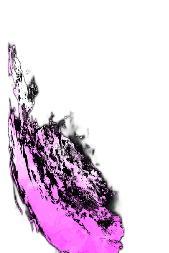
● As an example we can apply the ImageSaliencyFilter [ ] to an image (below) then ColorNegate[ ] (optionally Binarize[ ]) and then integrate; this gives you a more meaningful value of the integrals. The programmer can set the Saliency Method to orientation or contrast or intensity and the resulting image recommends the regions to apply the differential operators to. For the image below, it is the most salient region of the original image and if integrated can serve as the average saliency of the entire image.
What is a Monoidal Programming Language?
The Monoidal Language is a Turing compatible programming language with no syntax for conditionals e.g. if-else!
Indeed, the Wolfram Programming Language, in parts, is a Monoidal Language.
This inspiration came from Chapter 4 in [5] Bracewell’s book on computing with General Functions. Therein he explained that piecewise functions are difficult for analytical investigations and computations and best one make the entire function and all its operations into some monoidal form as he explained away in multiple General Functions e.g. Dirac Delta Function.
First I give a simple programming example in Wolfram Programming Language to motivate the programmers, then I code a few text examples in ceanolors[ ] monoid container.
Monoid version of if-else
This is an example of a nested if-else evaluator:
Which[θ>π/2,expr1,0<θ<π/2,expr2,True,expr0]
Boole[ ]
In[]:=
Boole[1/2<1]
Out[]=
1
In[]:=
Boole[1/2>1]
Out[]=
0
Our goal is by using the Boole[ ] transform the Which[ ] structure above to a multiplicative structure of the form * similar to any sum series. is a Boole[ ] expression and any other expression. EvaluatorIf ==1,evaluateandplaceintoasum Why?1. This is a universal expression in any programming language while this is not:
i
∑
c
i
expr
i
c
i
expr
i
c
i
expr
i
elseevaluatenothingorplacea0intoasum
a*expr1+b*expr2+c*expr3
Which[θ>π/2,expr1,0<θ<π/2,expr2,True,expr0]
These are simply for demo and studies, for now one operator but programmers can get used to the monoidal programming.
Glyph Symbols
Cloud Import AQUA-MODIS Ocean Colors scans
Review “/geophysical_data/chlor_a”
Cloud Import “/geophysical_data/chlor_a”
⧢ Color Separator Operator
TODO: If the 3D plot does not appear run it again, not sure why sporadically this happens.
Digression: Mona Lisa Over-Splined
TODO: If the 3D plot above does not appear run it again, not sure why sporadically this happens.
Clear initializes all monoid’s internal variables to their original presets.
Morphological Components
Image connected components, is a binary image segmentation technique that segments image foreground based on pixel connectivity. Simply put, partition an image or segment an image based upon the regions which are connected, and order this list from the largest number of pixels (area) to the smallest.
This Glyph-symbol acts like a prefix operator on the right-hand-side operand and groups the pixels of the image into components with certain geometrical meaning.
In case the image colonizations do not match, please run to access the original NASA variable namely
Segment Deletion
Multiply the original image by the mask to remove only those segments.
This Glyph-symbol acts like a prefix operator on the right-hand-side operand and clusters the pixels of the image.
⧈ : Σ Image Summation Operator
Σ is the usual summation operator but this time for images. Therefore if you ever have a list of images or segmentation list from a single image, then you can easily sum them up into a single image again.
References
[1] Chlorophyll a, Jeremy Werdell and John O’Reilly and Chuanmin Hu and Lian Feng and Zhongping Lee and Bryan Franz and Sean Bailey and Christopher Proctor
https://www.earthdata.nasa.gov/apt/documents/chlor-a/v1.0#abstract
[2] Aqua MODIS Level-2 Regional Ocean Color (OC) Data, version 2022.0
https://access.uat.earthdata.nasa.gov/collections/C1272940553-OB_CLOUD
[3] The Ocean Biology Processing Group (OBPG) produces a standard suite of ocean color products for all compatible sensors at Level-2 and Level-3, plus sea surface temperature (SST) products from MODIS and VIIRS. The OBPG also produces a suite of Level-3 evaluation products. The descriptions and references for these standard and evaluation products (provided below) are intended to satisfy the Algorithm Theoretical Basis Document (ATBD) requirement as defined by the NASA Earth Observing System Project Science Office.
All products produced by the OBPG are distributed and archived by the Ocean Biology Distributed Actice Archive Center (OB.DAAC).
https://oceancolor.gsfc.nasa.gov/resources/atbd/
[4] OB.DAAC
Ocean Biology DAAC
https://www.earthdata.nasa.gov/centers/ob-daac
[5] R. Bracewell The Fourier Transform and Its Applications. MacGrawHill