Derivating things Construction of the Generalized functions and computing their derivatives (fully coded)
Part1-ν2.1
Dara O Shayda
dara@compclassnotes.com
dara@compclassnotes.com
In[]:=
DateObject[]
Out[]=
Abstract
Je code donc je fais des math: I code therefore I math! 100% live code training scripts for advanced topics in the theory and techniques of the Generalized functions namely the derivatives of |x|, ||x||, Λ[x], Π[x] and deriving the δ[x] and its derivatives + all their Fourier series and their derivatives’. You will train on how to code and develop advanced symbolic computing programs to define and derive and visualize the construction of the Generalized functions while enforcing their properties. While developing the Lagrangian for the Hexapod robot and molecular ring and chain structures I was faced with the challenge of adding Abs[ ] based terms into the resulting Lagrangian due to the Norm[ ] or Sqrt[ ] associated with elastic joints or ball-spring models which required a non-zero spring position; moreover apropos of the Hexapod due to the signals required to actuate motion in the elastic joints more complex derivative discontinuities had to be constructed in the control code. The basic bottom line was that I had to quickly train to take derivatives of discontinuous functions or functions with discontinuous derivatives and plug them into super large systems of differential equations. I found the modern literature on the required topics worthless, so I turned my attention to older publications around the 1950s to 1960s and therefore set out to code all that was devised and discovered and applied to advanced differential equations e.g. derivatives of Heaveside functions to acquire the Dirac Delta function. If you are a spirited STEM kid or instructor trying to program a multi-pod robot controller or you are a first year chemistry student advancing your training in molecular dynamics, you want to learn these topics so you are no lesser than others. The techniques and symbolics and formalism are that of the Bracewell [1], I used the Lighthill [2] for rigour and more detailed and accessible formalism. For undergraduates and those seeking intuitive but rigorous understanding Bracewell [1] is the man!Live Code Notebook:https://www.wolframcloud.com/obj/ccn2/Published/derivating_things_part1.nb math, mathingverb-The act of preforming mathematics (shortened word: math)Usage:- “Shhh! Hold on, I’m mathing!!”- “... now I need to math all over again ”- “Gauss as a child was really mathed up!” ⟵ mine
Sources: https://www.mathnasium.com/ca/blog/20151016-word-of-the-day-mathing https://www.urbandictionary.com/define.php?term=mathinghttps://www.powerthesaurus.org/mathing/definitions In case of bugs in the code or the theory please make contact to fix ASAP. Keywords: Lagrangian mechanics, Lagrangian linear operator, derivative, Generalized functions, Heaveside functions, Dirac Delta functions, LogisticSigmoid functions, Fourier series, Taylor series.
100% Fat Free Mathematics

Software
Release: ν2.1
Scripts: Symbolic computations performed in Wolfram Mathematica 14.3 .Notebook: https://www.wolframcloud.com/obj/ccn2/Published/derivating_things_part1.nb Support: Contact the author for additional code, bugs, correction in maths and algebraic/mathematical mistakes or invalid inferences.Nomenclature: Most functions and most identifiers start with lower case letters, all native vendor identifiers start with upper case. No Packaging: There is no software engineering applied to the code here nor elsewhere in the author’s technical notes to reduce the difficulties and version mismatches in future. The eager readers can simply copy paste the code or download and run the notebook. TODO: 1. Create additional all code parts dealing with certain advanced techniques in Generalized functions and systems of differential equations solvers, however focused on particular families of equations for particular applications2. Add integration and Integral equations for the same Generalized functions 3. Add partial differentiation for 2D and 3D imagesTOLEARN:1. Generalized functions used in Feynman’s and Dirac’s physics computations. Duplicate the exact computations and possibly set forth some new computing and results. Known Issues:
© 2012-Present CCN StudiosCreative Commons Attribution-NonCommercial-ShareAlike 4.0

Initialization
In[]:=
Notation`AutoLoadNotationPalette=False;Needs["Notation`"];ClearNotations[];CloudGet["https://wolfr.am/1xEVtfjBx"];ℋinit[];
version: β6.1
Apercu: Impulse Function ☺ ⟶ Impulse Symbol
?
Impulse Function
Before we do anything, per Bracewell [1], we define the shape and the algebra of an Impulse function in an intuitive manner and yet with some code:
Definition: Generally an Impulse function is firstly, an infinite series of mathematical functions with compact support (they evaluates to zero outside of these compact sets). Second, their integrals along the Real line is +1. Third, their derivatives integral along the Real line is 0.
compact support : for an informal definition, imagine the lengths/areas/volumes/measures of regions wherein the function is non-zero are finite quantities and there is finite number of such regions. Therefore their total sum is also finite. (special case)
integrals along the Real line is +1 : It is similar to a probability or density distribution.
derivatives integral along the Real line is 0 :
impulse⟶
n
compact support : for an informal definition, imagine the lengths/areas/volumes/measures of regions wherein the function is non-zero are finite quantities and there is finite number of such regions. Therefore their total sum is also finite. (special case)
integrals along the Real line is +1 : It is similar to a probability or density distribution.
derivatives integral along the Real line is 0 :
First attempt at an Impulse Function
In[]:=
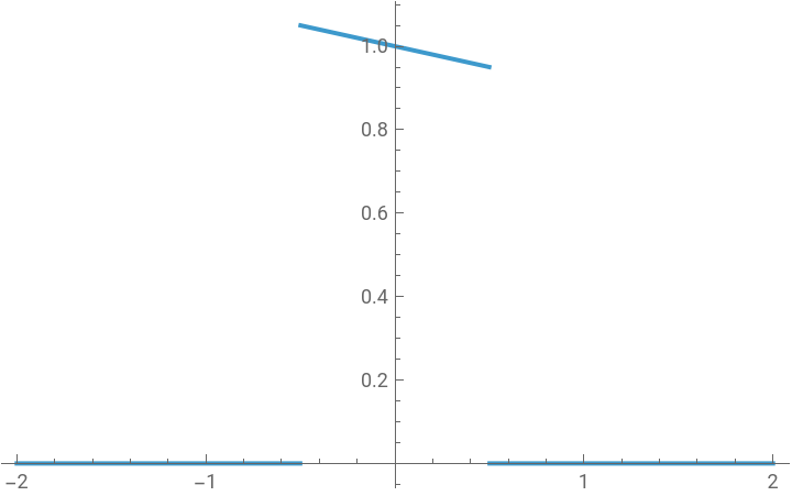
impulseFunction[x_]:=Piecewise[{{0,x<-1/2},{-0.1*x+1,-1/2<=x<=1/2},{0,x>1/2}}]
In[]:=
TraditionalForm@impulseFunction[x]
Out[]//TraditionalForm=
|
In[]:=
Plot[impulseFunction[x],{x,-2,2}]
Out[]=
In[]:=
Integrate[impulseFunction[x],{x,-∞,∞}]
Out[]=
1.
The integral of the derivative is non-zero and therefore not a good candidates, reasons for this condition will be discussed later:
Second attempt: Unit Step
Q: What is it called Impulse?
A: It acts like a signal, or better to say a filter, multiply this Impulse by any function and it returns the segments of the function that are within its compact support. The latter means it filters out the part of the function where its support is 0.
Pictorial filtering(s) below should be useful.
A: It acts like a signal, or better to say a filter, multiply this Impulse by any function and it returns the segments of the function that are within its compact support. The latter means it filters out the part of the function where its support is 0.
Pictorial filtering(s) below should be useful.
Make a narrower and taller Impulse function
All properties hold:
Slide the Impulse function:
Multiply the very narrow Impulse function by any function , below Cos[ ] and it will return approximately the Cos[0] or in general the f[0] .
Slide the Impulse function and take its integral multiplied by a functions e.g. Cos[x] and this time the integral returns the value Cos[0.01] the new location the apex of the Impulse function was moved to:
Impulse Symbol!? and Why?
See section 5 for the How? with more detailed elucidations and computations, however briefly here:
● When we took some integrals, we actually were lucky we could use one single integral, but that one integral is actually the limit of infinitely my integrals inching towards a final limit
● The difference quotient for Abs[ ] does not have a limit in the complex plane:
To handle this difficulty in differential equations and any applications of derivatives of Abs[ ] or Norm[ ] or Sqrt[ ] , Mathematica introduced RealAbs with the following property:
or
or
In construction of families of sequences to define the Dirac Delta functions, the very shape of the thinner and taller impulse functions is of no importance as long as the properties of the δ[x] are maintained:
Arg[z] the Menace!
1.1 Detailed derivation: along x-axis in complex plane
● No limit at (x, y) due to the terms a and b!
1.2 Detailed derivation: along the Real line
● Let’s assume x is Real
● Multiplied numerator and denominator by Abs[x+h]+Abs[x]) and Inactive[Abs[x+h]+Abs[x]] both terms are positive. The Inactive[ ] is used to aid with the fractional custom cancellations:
● Manually removed the Abs[ ] from the squared terms:
● Put the terms back together into a single quotient and apply the function Activate[ ] :
● Separate into two quotients again:
● Take the limit:
1.3 Fourier Expansion of Abs[ ]
1.4 Fourier expansion to define a derivative at 0
Make incredibly snugger approximation:
Plot error function:
1.5 Briefest ever Taylor Expansion of Abs[ ]
1.8 Fourier expansion to define a derivative at 0
1.9 Integrate the Fourier expansion for a new Abs[x] approximation with derivative at 0
This is a round about way approach, more on the experimental side of these computations and ideas.
Create a constant variable c for the integral of the Fourier expansion above that approximated the derivative of Abs[x]:
Create a constant variable c for the integral of the Fourier expansion above that approximated the derivative of Abs[x]:
Replace the c, the constant of of integration, with its solution above:
1-D
In 1-D case the Pythagorean theorem is simplified and the squared terms replaced with Abs[ ] terms and no matter what simplification strategy they linger.
Guideline: Always replace Abs with RealAbs
2-D
3-D
HeavisideLambda[ ] or Triangle distribution:
Normally we work with a translation to start at (0,0) at time 0:
3.1 Distribution???
This Triangle thing acts like a probability distribution:
3.1.1 PDF
3.1.2 CDF
3.2 Translate the triangle to get y=0 at x=0
Translate the triangle anywhere you like to impact as a signal:
3.3 Fourier expansion to define a derivative at 0
3.4 Dipole: Derivate the Triangle
This shape of a positive hump for negative x values and then immediately after passing through the 0 appears the same jump multiplied by -1 (upside down?) is called Dipole shape [1]:
3.5 Derivate the Fourier expansion of the Triangle
3.6 Smooth Dipole
4. Ideation: Infinitesimal Dipole
Concept is from Bracewell[1] wherein the author used the dipole pictorials to create an intuition that later would be transferred to mathematical expressions. I did alter the implementation to match the rest of the coding here.
Best to read section 5 first.
Best to read section 5 first.
● Gaussian kernel is from the Lighthill [2]:
● Increasing function of n for height at 0
● Distribution property holds:
● Sifting proper holds as well:
● Integral of the kernel’s derivative is 0:
4.1 Dipole: The kernel’s derivate
4.2 Symbolics: Power operators
● Initialize the operators:
4.3 Construct an Infinitesimal Dipole with Dirac Delta Function
● Compute two Fourier series for Dirac Delta function , one located before the origin and one after
● Multiply the Gaussian kernel by the dipole to smoothly filter out the periodicity of the Fourier series:
● The periodicity of the Fourier expansion, while an issue for the mathematical formalisms, is not an issue for applying the Fourier expansions of Dirac Delta in physical systems since the Lagrangian dealing with such systems deal with small angles and even smaller variations.
Symbols vs. Functions
Read this section after you have read the rest of the Dirac Delta construction process below. There are mathematical functions as you understand in modern mathematics. There are lesser known entities called Symbols or Generalized functions. These are entities that are not functions and yet they behave like unto functions when used in Expressions and Equations and their algebras.
The most stunning attribute of Bracewell [1] is his English adumbration(s) of the formal systems and the symbols and interrelations to the physics and and the fact that in reality much of the physics formalism does not exist in our physical reality e.g. Point mass or Point charge and definitely Dirac Delta Impulse Symbol.
In comparison to his writings, today’s Physics publications read like comic novels!
Therefore, mid writing this technical note, I decided to scrap my verbiage and rely on Bracewell’s [1] in an attempt to parallel his narrative and symbolism. This was my form of learning from him, per advice of Von Neumann to treat learning mathematics like learning a new foreign language.
Note: Plots are unnaturally scaled to match the screen sizes.
Note: HeavisidePi[ ] in place of UnitBox[ ], since the HeavisidePi[ ] can participate in all integral and differential equations while UnitBox[ ] cannot due to lack of derivatives at its corners.
5.1 Do the calculus things to compute the derivative of H[x]
5.2 Difference Quotient for derivative computation
The boxes below grow higher and higher but due to the size of their height and this limited screen size they look capped!
Test the integral of the difference quotient for small range:
All the way along the Real line:
And that Derivative of the H[x] function is indeed the Dirac Delta, the Impulse Symbol, impersonating a function:
5.3 Sifting Property
Make a funky f function:
Integrate from -2τ to +2τ which if a fantastic narrow range to help the NIntegrate[ ] function to compute with enough accuracy:
5.4 Fourier expansion of the Dirac Delta function
Q: Why in the world do I need to compute the Fourier expansion of the Dirac Delta function?
A1: Per Bracewell [1] in section 1 of this technical notebook, the shape of the so-called box functions does not matter, what matters is whether their integral identities hold, hence replacing the Dirac Delta function. Therefore, the weird wavy Fourier expansion is a good test of the idea.
A2: We need to be able to compute the derivative values of the Dirac Delta function at 0. And that is not possible due to undefined value at 0. However, a Fourier expansion always returns a value with a predictable error.
The following Cosine Fourier series does not compute since the HeavisideTheta[0] is undefined, see the following evaluation and plot:
Evaluate the FourierCosSeries [ ] again and all work and evaluate:
or
5.6 Sifting Property
Test this identity with Mathematica:
5.7 Dipole: Derivative of the Fourier expansion of the Dirac Delta function
5.9 Why Fourier expansion of the Dirac Delta function!|
Q: Why in the world do I need to compute the Fourier expansion of the Dirac Delta function?
A1: Per Bracewell [1] in section 1 of this technical notebook, the shape of the so-called box functions does not matter, what matters is whether their integral identities hold, hence replacing the Dirac Delta function. Therefore, the weird wavy Fourier expansion is a good test of the idea.
A2: We need to be able to compute the derivative values of the Dirac Delta function at 0. And that is not possible due to undefined value at 0. However, a Fourier expansion always returns a value with a predictable error.
A1: Per Bracewell [1] in section 1 of this technical notebook, the shape of the so-called box functions does not matter, what matters is whether their integral identities hold, hence replacing the Dirac Delta function. Therefore, the weird wavy Fourier expansion is a good test of the idea.
A2: We need to be able to compute the derivative values of the Dirac Delta function at 0. And that is not possible due to undefined value at 0. However, a Fourier expansion always returns a value with a predictable error.
● The derivative of Heaviside unit-box or Π[x] or HeavisidePi[x] is merely subtraction of two Dirac Delta functions! (-δ1 - δ2)
References
1. Ronald Bracewell , The Fourier Transform & Its Applications, McGraw-Hill Science
2. MJ. Lighthill, Introduction to Fourier Analysis and Generalized Functions
2. MJ. Lighthill, Introduction to Fourier Analysis and Generalized Functions