OCEAN COLOR CalculusNASA MODIS-Aqua Satellite Image Data(fully coded)
Part 1-α8.0
Dara O Shayda
dara@compclassnotes.com
dara@compclassnotes.com
In[]:=
DateObject[]
Out[]=
Abstract
This live code notebook is a specific exercise for creating monoidal-like custom language to provide image calculus e.g. derivatives for images and their corresponding data. And in particular the focus of the data sources is NASA’s Ocean Color satellites e.g. Modis-Aqua. is the name of the monoid-like container that acquires data from NASA’s cloud systems and process the data into images and provide bona fide calculus by first Spline the images and then apply partial derivatives to the image Splines. The language is designed with an eye on for training and as a matter of fact provides unlimited examples of differential structures to investigate and understand the differential operators in . The calculus is further endowed with image process and machine learning algorithms e.g. Perona-Malik filters applied to the pixel Clusters in a single image. The output images result in better understanding of the nature of the target scanned area of the oceans and the particular data e.g. surface temperature or the scrubbing by the aquatic microbial organisms (coming soon). Note: More of these live notebooks will be released for a variety of variables and ocean regions, notebooks become too large and therefore each variable requires a notebook of its own.
ceanolors[]
3
CO
2

Software
Release: α8.0 .

Scripts: Symbolic computations performed in Wolfram Mathematica 14.3 .Notebook: https://www.wolframcloud.com/obj/ccn2/Published/Aqua_Modis_ocean_colors1.nb Support: Contact the author for additional code, bugs, correction in maths and algebraic/mathematical mistakes or invalid inferences.Nomenclature: Most functions and most identifiers start with lower case letters, all native vendor identifiers start with upper case. No Packaging: There is no software engineering applied to the code here nor elsewhere in the author’s technical notes to reduce the difficulties and version mismatches in future. The eager readers can simply copy paste the code or download and run the notebook. TODO: 1. Full JSON ASCII output support for third party Python, JS, C/C++/C# programs.2. Image derivatives are taken on the grey level version of the image, in case the derivatives ought to be taken for each channel.3. One or several Cloud Objects containing the file, its monoids and parametrizations with API Functions for external interactions.This is critical and urgent to allow for large number of variables and scans while the size of the live code notebook would remain small. 4. Login, authorization and Hash for time-stamping and copyrights. 5. Interim images and other related data and computations saved into cloud objects.6. Integration over an image7. PDE solutions over one image and over a family of images.8. Wavelets9. Volumetric or 3D image versions and animation flip-books TOLEARN:1. Color maps that match the coloration of the ocean waters as seen by the satellites 2. Animate regions of oceans Known Issues:1.
© 2012-Present CCN StudiosCreative Commons Attribution-NonCommercial-ShareAlike 4.0

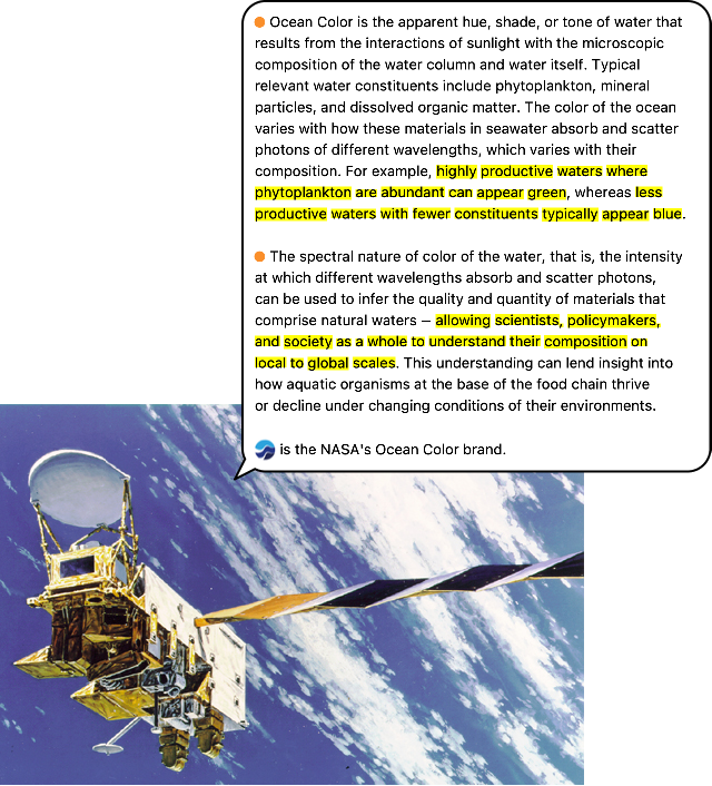
What is Ocean Color?
Out[]=
ceanolors[ ]
Monoidal Container
Monoid: In abstract algebra, a branch of mathematics, a monoid is a set equipped with an associative binary operation and an identity element. For example, the nonnegative integers with addition form a monoid, the identity element being 0.
Container: A habitat for programs to reside within, in and of themselves fully functioning, with no essential external environment support or any additional resources, and sheltered regardless of the outside environment. Container has cloud I/O services which allows communications with standard commercial third party software.
For example, NASA’s satellite image/scan file “AQUA_MODIS.20260111T000000.L2.SST4.NRT.nc” is just that ,namely a file!
container makes that mere file into a Container:
● Imbues the file with a monoidal Infix, Prefix, Postfix operators, behave much like the arithmetic operators +, -, * and = .
● Splines to parametrize the discrete images so operators e.g. partial derivatives or Integrations can seamlessly apply .
● TODO: One or several Cloud Objects containing the file, its monoids and parametrizations with API Functions for external interactions
● TODO: Login, authorization and Hash for time-stamping and copyrights.
● TODO: Interim images and other related data and computations saved into cloud objects.
Container: A habitat for programs to reside within, in and of themselves fully functioning, with no essential external environment support or any additional resources, and sheltered regardless of the outside environment. Container has cloud I/O services which allows communications with standard commercial third party software.
For example, NASA’s satellite image/scan file “AQUA_MODIS.20260111T000000.L2.SST4.NRT.nc” is just that ,namely a file!
ceanolors[]
● Imbues the file with a monoidal Infix, Prefix, Postfix operators, behave much like the arithmetic operators +, -, * and = .
● Splines to parametrize the discrete images so operators e.g. partial derivatives or Integrations can seamlessly apply .
● TODO: One or several Cloud Objects containing the file, its monoids and parametrizations with API Functions for external interactions
● TODO: Login, authorization and Hash for time-stamping and copyrights.
● TODO: Interim images and other related data and computations saved into cloud objects.
Initialization
In[]:=
Notation`AutoLoadNotationPalette=False;Needs["Notation`"];ClearNotations[];CloudGet["https://wolfr.am/1BKwPgFcC"];ceanolors[]
Out[]=
Version α8.0x,y,xy,yx,xx and yy are protected.,
Aquatic Image & Data Acquisition
● First you need to identify the satellite scan identifier (product as coined by NASA) and preferably assign it to a variable .● Paradigm: satellite’s components; as you say phrases such ocean’s colors the monoidal container allows for such Free Form Spoken Language. ● ‘s access, see below, is mandatory for the s monoidal container which obtains the “attributes” of the specific satellite scan or NASA’s product . ● An internal symbol holds the value of a handle to the parsed .nc formatted data No files! The .nc scans are stored into the cloud objects or in the local memory of the local machine and no files or even interim files.
ceanolors[]
ceanolors[]'
In[]:=
scan="AQUA_MODIS.20260111T000000.L2.SST4.NRT.nc";
:scan's"attributes"
Out[]=
{/,/geophysical_data,/geophysical_data/bias_sst4,/geophysical_data/flags_sst4,/geophysical_data/l2_flags,/geophysical_data/qual_sst4,/geophysical_data/sst4,/geophysical_data/sstref,/geophysical_data/stdv_sst4,/navigation_data,/navigation_data/latitude,/navigation_data/longitude,/navigation_data/tilt,/processing_control,/processing_control/flag_percentages,/processing_control/input_parameters,/processing_control/qual_sst4_percentages,/processing_control/sst4_flag_percentages,/scan_line_attributes,/scan_line_attributes/clat,/scan_line_attributes/clon,/scan_line_attributes/csol_z,/scan_line_attributes/day,/scan_line_attributes/detnum,/scan_line_attributes/elat,/scan_line_attributes/elon,/scan_line_attributes/msec,/scan_line_attributes/mside,/scan_line_attributes/slat,/scan_line_attributes/slon,/scan_line_attributes/time,/scan_line_attributes/year,/sensor_band_parameters,/sensor_band_parameters/aw,/sensor_band_parameters/bbw,/sensor_band_parameters/F0,/sensor_band_parameters/k_no2,/sensor_band_parameters/k_oz,/sensor_band_parameters/Tau_r,/sensor_band_parameters/vcal_gain,/sensor_band_parameters/vcal_offset,/sensor_band_parameters/wavelength}
Get the (meta)data attached to every variable:
ceanolors[]
Access the long_name Key/Attribute to get a short summary of what the data contains:
Try another variable:
Access the long_name Key/Attribute to get a short summary of what the data contains:
From here and onward all computations are for the variable “/geophysical_data/sst4”, which are surface temperature related:
*: Commutative multiplication operator
* scales the image or whatever other structures as multiplicands from right or left hand sides.
One remedy for the non-black background, is to alter the number of Quantiles used as a source of interpolation for color adjustment, in the case of this particular satellite image the number if set to 2, the background computes to 0.
⧈ : Image Calculus
⊗ : Commutative multiplication operator
⧢ Color Separator Operator
🕶 Unit Interval Rescale Operator
⊕ , ⊖ : Arithmetic operators
Remove the Blue and Red colors:
To measure the distance between two images use the grouping operator ‖ as follows:
Remove the Blue and Green colors:
Remove the Green and Red colors:
⌐ Color Negate Operator
◐ Binarize Operator
Color Machine Learning
“filter” computes a smoothed out clustering while preserving the “ridges” between neighboring regions. In particular the default filer is set to the Perona-Malik diffusion algorithm. More than often the satellite images are too busy for the cluster to form meanings and best to diffuse the image first prior to the same clustering algorithm.
Multivariate Calculus: Image Derivatives
This is a simple example of an image derivative to get used to the general concepts and the outputs and relate the outputs to regular understanding of the derivatives.
First create an image which along the x-axis is constant in pixel values and yet along the y-axis varies smoothly e.g. as a Gaussian distribution function.
As you can see the Gaussian bell is the white area towards the bottom of the image. Note that the pixel values are mapped onto the [0, 1].
As you can see a black image obtained for the derivative along the x-axis:
Let us take the derivative of the original Gaussian function:
Plot and we see the previous white area is now halved by the dip caused by the derivative’s negative values. Note that the pixel values are mapped onto the [0, 1]. Therefore the negative valued region is now a dip namely y values around 0.5 to 0.
Direct Access to the Spline Functions
Derivative of the image Spline is again another Spline:
Monoidal Calculus
ceanolors[ ] ⟷ Wolfram
References
[1] Aqua MODIS Level-2 Regional Ocean Color (OC) Data, version 2022.0
https://access.uat.earthdata.nasa.gov/collections/C1272940553-OB_CLOUD
[2]: “/geophysical_data/sst4” (click on the Variables link)
https://cmr.earthdata.nasa.gov/search/concepts/C1615934239-OB_DAAC.html
https://access.uat.earthdata.nasa.gov/collections/C1272940553-OB_CLOUD
[2]: “/geophysical_data/sst4” (click on the Variables link)
https://cmr.earthdata.nasa.gov/search/concepts/C1615934239-OB_DAAC.html