This notebook extends the well-known Wigner function, originally defined as a phase-space representation for a single mode, to the two-mode case. The joint Wigner function depends on four phase-space coordinates , , , ), making it inherently a 4D object that cannot be plotted directly. To study it, we examine lower-dimensional slices (2D or 3D cuts) or compute marginal distributions obtained by integrating over selected variables.
(
x
1
p
1
x
2
p
2
In[]:=
PacletInstall[CloudObject["https://wolfr.am/DevWQCF"],ForceVersionInstall->True]<<Wolfram`QuantumFramework`<<Wolfram`QuantumFramework`SecondQuantization`
Out[]=
PacletObject

Read this for MaTEX installation: https://www.wolframcloud.com/obj/nikm/Published/TikZ.nb
Definition of Joint Wigner Function
Definition of Joint Wigner Function
One way to define the joint Wigner function for two modes 𝑎, 𝑏 is through a trace expression that depends on the displacement and phase-shift (parity) operators. Explicitly, it can be written as:

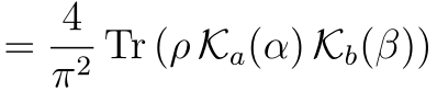
For convenience, this expression can be rewritten in terms of a new family of operators defined as: with

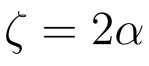
And the associated matrix elements are:where

operators implementation:
In[]:=
ClearAll[,mn];mn[γ_,{m_,n_}]:=Chop@N@With{ζ=2γ},Exp-Ifm>=n,LaguerreL[n,m-n,],LaguerreL[m,n-m,][γ_,size_:$FockSize]:=[γ]=Outer[mn[γ,{#1,#2}]&,Range[0,size-1],Range[0,size-1]]
n
(-1)
2
Abs[ζ]
2
n!
m!
m-n
ζ
2
Abs[ζ]
m!
n!
n-m
Conjugate[-ζ]
2
Abs[ζ]
Numeric compiled version of :
mn
Kmncomp=FunctionCompile[Function[{Typed[γ,"ComplexReal64"],Typed[m,"Integer64"],Typed[n,"Integer64"]},Module[{ζ,res},ζ=2.0*γ;res=If[m>=n,Sqrt[Gamma[n+1.0]/Gamma[m+1.0]]*ζ^(m-n)*LaguerreL[n,m-n,Abs[ζ]^2],Sqrt[Gamma[m+1.0]/Gamma[n+1.0]]*Conjugate[-ζ]^(n-m)*LaguerreL[m,n-m,Abs[ζ]^2]];(-1)^n*Exp[-Abs[ζ]^2/2.0]*res]]];
Joint Wigner definition:
In[]:=
wigner2mod[ρ_,α_,β_]:=Trρ.KroneckerProductα,
4
2
π
ρ["Dimensions"][[1]]
,β,ρ["Dimensions"][[2]]
Faster versions without explicit trace( gain will depend on how sparse the density matrix is):
In[]:=
ClearAll[NWigner2mod]NWigner2mod[rho_SparseArray,α_,β_]:=Withd=)Dotvals,Kmncomp[α,Quotient[#2-1,d],Quotient[#1-1,d]] Kmncomp[β,Mod[#2-1,d],Mod[#1-1,d]] &@@@pos
First[rho["Dimensions"]]
,vals=rho["ExplicitValues"],pos=rho["ExplicitPositions"],(4./2
π
In[]:=
ClearAll[Wigner2mod]Wigner2mod[rho_SparseArray,α_,β_]:=Withd=)Dotvals,mn[α,{Quotient[#2-1,d],Quotient[#1-1,d]}] mn[β,{Mod[#2-1,d],Mod[#1-1,d]}] &@@@pos
First[rho["Dimensions"]]
,vals=rho["ExplicitValues"],pos=rho["ExplicitPositions"],(4/2
π
Timing when the density matrix has a high degree of sparsity(notable gain)
In[]:=
SetFockSpaceSize[20];
In[]:=
ρ=FockState[{1,0}]["DensityMatrix"];
“Naive” definition:
In[]:=
wigner2mod[ρ,0.2,1.]//RepeatedTiming
Out[]=
{0.0296498,-0.0425311}
Using the numerical version:
In[]:=
NWigner2mod[ρ,0.2,1.]//RepeatedTiming
Out[]=
{0.0000111991,-0.0425311+0.}
Time gain:
In[]:=
%%[[1]]/%[[1]]
Out[]=
2647.51
Visualizing Fock states |m,n〉
Visualizing Fock states |m,n〉
Analytical expression for |m,n〉 states:
In[]:=
wignerFock[{α_,β_},{m_,n_}]:=LaguerreL[m,4Abs[α]^2]LaguerreL[n,4Abs[β]^2]Exp[-2(Abs[α]^2+Abs[β]^2)]
4
π^2
m+n
(-1)
Compare result of Wigner2mod with state |1,0〉 analytical result:
In[]:=
With[{ρ=FockState[{1,0},8]["DensityMatrix"]},Simplify[wignerFock[{α,β},{1.,0}]==Wigner2mod[ρ,α,β]]]
Out[]=
True
Density matrices for states |m,0〉:
In[]:=
SetFockSpaceSize[8];ρs=Array[FockState[{#,0}]["DensityMatrix"]&,6];
Spatial range:
In[]:=
range=N@Subdivide[-2,2,21];
Choose sampling of points for 3D slices :
(=0)
p
2
In[]:=
sampsFock=TableFlattenTablex1,p1,x2,NWigner2modρs[[i]],,,{x1,range},{p1,range},{x2,range},2,{i,6};
x1+p1
2
x2
2
Plot the 3D slices:
In[]:=
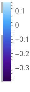
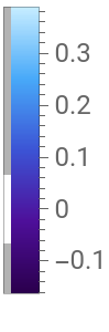
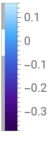
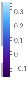
Grid@Partition[Table[ListDensityPlot3D[sampsFock[[n]],ColorFunction->"DeepSeaColors",PlotLegends->Automatic,AxesLabel->{"","",""},LabelStyle->12,PlotLabel->StringForm["State : |``,0〉",n],RegionFunction->(Not[#1>0&<0]&)],{n,6}],2]
x
1
p
1
x
2
Out[]=

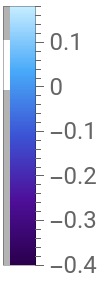

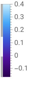




Additional Examples of two-mode Joint Wigner Function
Additional Examples of two-mode Joint Wigner Function
NOON State
NOON State
In[]:=
SetFockSpaceSize[10];
NOON state with N = 4:
In[]:=
ρ=(FockState[{4,0}]+FockState[{0,4}])["DensityMatrix"];
1
2
3D slices :
(=0)
p
2
Visualize the 3D slices:
Entangled cat state
Entangled cat state
Set up spatial grid:
Evaluate the function:
Visualize the 3D structure:
Visualize slice density plots along z planes, some slices look resemble the density plot of the one mode cat state signaling non classical behavior:
Bright state
Bright state
A bright state is obtained when = n:
Pick bright state with = n = 4:
Wigner function in terms of symbolic variables:
Visualize the 3D slices:
X slices visualization:
Averages and marginals
Averages and marginals
Let’s use the symbolic function we got from the last example:
Plot the marginal:
Define a NOON state with π phase (we can use the definition of collective states):
Density matrix:
Calculate the 4D symbolic function of the phase space variables:
The analytical result is:
First mode operators:
Second mode operators(specify the order):
Bracket result:
Same result as expected, however, the Wigner function approach can be use for more complicated function of the phase space variables.
CITE THIS NOTEBOOK
CITE THIS NOTEBOOK
Two-mode phase space representation: joint Wigner function
by Bruno Tenorio
Wolfram Community, STAFF PICKS, September 8, 2025
https://community.wolfram.com/groups/-/m/t/3542358
by Bruno Tenorio
Wolfram Community, STAFF PICKS, September 8, 2025
https://community.wolfram.com/groups/-/m/t/3542358