In this notebook, i show an implementation of a recent paper Murtadho, T., Cataldini, F., Erne, S., Gluza, M., Tajik, M., Schmiedmayer, J., & Ng, N. H. Y. (2025). Measurement of total phase fluctuation in cold-atomic quantum simulators. Physical Review Research, 7(2), L022031. https://doi.org/10.1103/PhysRevResearch.7.L022031 in Wolfram Language. The simulations do not include the experimental part of the research, but the main point is demonstrating and validating the technique for total phase extraction. This approach could be applied to the measurement of correlations in both one-dimensional condensates and two-dimensional bilayer systems.
Read this for MaTEX installation: https://www.wolframcloud.com/obj/nikm/Published/TikZ.nb
Two Parallel 1D Quasi-condensates
Two Parallel 1D Quasi-condensates
Two adjacent quasi-condensates can be modelled by a bosonic field operator:

(
1
)withandbeingphaseanddensityfields
ϕ
a
n
a
Total phase field:

(
2
)Linearization of continuity equation for total density for irrotational currents:

(
3
)Using some approximation it is possible to express Equation (3) as a Poisson equation for the total phase, in the paper they also impose equal mean densities for the two condensates. But in their analysis they also include how to model the case of unequal densities
Simulation Parameters
Simulation Parameters
Physical Constants
Physical Constants
In[]:=
hb=QuantityMagnitude@UnitConvert["ħ","Joule*Second"];kB=QuantityMagnitude@UnitConvert[Quantity["BoltzmannConstant"],"Joules/Kelvin"];mRb=QuantityMagnitude@UnitConvert["AtomicMass"],"Kilograms";
Traps and interaction
Traps and interaction
In[]:=
ωperp=2π1400;(*radialtrapfrequency*)
In[]:=
aS=5.210^-9;(*s‑wavescattering[m]*)
In[]:=
g1D=2hbωperpaS;(*effective1‑Dcoupling[J·m]*)
Simulation grid
Simulation grid
In[]:=
L=10010^-6;(*systemlength[m]*)Nz=801;(*gridpoints*)dz=L/(Nz-1);zGrid=N@Subdivide[-L/2,L/2,Nz-1];(*totalzdomain*)bulkIndex=With[{l=Abs[zGrid]-40},Flatten@Position[l,Min[Abs[l]]]];(*indicesdeterminingthebulk*)NBulk=First[Differences@bulkIndex+1];(*numberofbulkpoints*)
-6
10
Other parameters
Other parameters
In[]:=
n0=15010^6;(*lineardensity[m^-1]*)pMax=50;(*fouriercutoff*)kList=2π/LWith[{l=Range[pMax]},Join[-Reverse@l,l]];(*Temperatureoftotalandrelativesector*)Tplus=5010^-9;(*Kelvin*)Tminus=3010^-9;(*Kelvin*)(*Timeofflight*)τ=1110^-3;(*seconds*)τ2=16;λτ[τ_]:=Sqrt[hbτ/(2mRb)];(*dynamicallength(m)*)nShots=1000;(*Numberofsingle‑shotrealisations*)d=2;(*distancebetweencondensate(m)*)EkList=(hb^2kList^2)/(2mRb);(*free-particleenergy*)epsList=Sqrt[EkList(EkList+g1Dn0)];(*Bogoliubovdispersionε_k*)sqrtERatio=Sqrt[epsList/EkList];(*√(ε_k/E_k)*)planeWaveMatrix=Exp[IOuter[Times,kList,zGrid]];(*Dimensions:{2pMax,Nz}*)
-3
10
-6
10
Sampling in-situ fluctuations fields
Sampling in-situ fluctuations fields
Phase fluctuations
Phase fluctuations
Sampling fluctuations from Bogoliubov modes:

(
4
)where =(g) is the Bogoliubov spectrum, =2m is the free dispersion, g ≈ 2 ℏ is the 1D interaction strength and is the scattering length. The summation is done along non zero integers {-pMax, pMax}
ϵ
k
E
k
E
k
n
0
E
k
2
(ℏk)
ω
⟂
a
s
a
s
In[]:=
samplePhaseFluctuations[T_,meanDensity_,scaleFactor_:1]:=Module{ηk,bkList,ξR,ξI,prefactors,phaseField},ηk=1.0(Exp[epsList/(kBT)]-1.0);ξR=RandomVariate[NormalDistribution[0,1],2pMax];ξI=RandomVariate[NormalDistribution[0,1],2pMax];bkList=Sqrt[ηk/2.0](ξR+IξI);prefactors=sqrtERatiobkList;phaseField=2Re[prefactors.planeWaveMatrix];scaleFactorphaseField
1
2meanDensityL
In[]:=
SeedRandom[100];
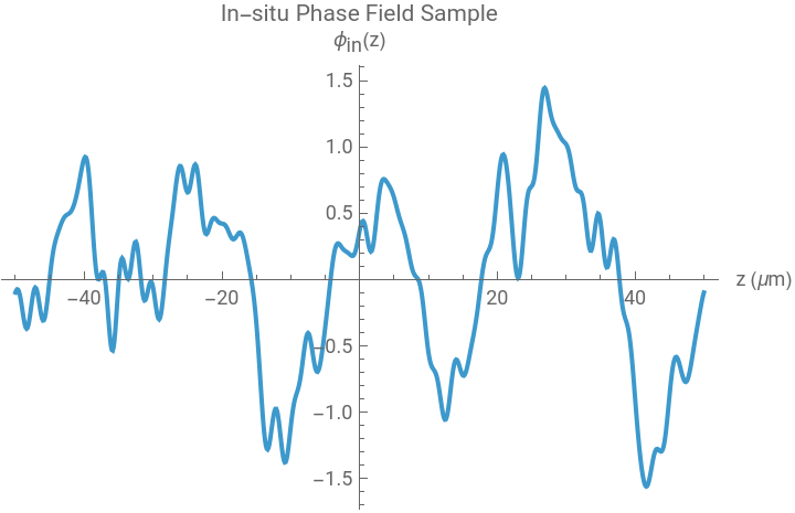
Sample phase fluctuations:
In[]:=
ϕsample=samplePhaseFluctuations[Tminus,n0/2];
Plot the sample:
In[]:=
ListLinePlot[Transpose[{zGrid*10^6,ϕsample}],AxesLabel->{"z (μm)","(z)"},PlotLabel->"In-situ Phase Field Sample",PlotRange->All]
ϕ
in
Out[]=
Density fluctuations
Density fluctuations
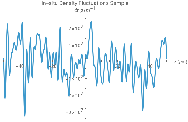
In a similar way the density fluctuations can be defined:

(
5
)In[]:=
sampleDensityFluctuations[T_,meanDensity_,scaleFactor_:1]:=Module{ηk,bkList,ξR,ξI,prefactors,densityField},ηk=1.0(Exp[epsList/(kBT)]-1.0);ξR=RandomVariate[NormalDistribution[0,1],2pMax];ξI=RandomVariate[NormalDistribution[0,1],2pMax];bkList=Sqrt[ηk/2.0]*(ξR+IξI);prefactors=sqrtERatio*bkList;densityField=2Re[prefactors.planeWaveMatrix];scaleFactordensityField
2meanDensity
L
Sample density fluctuations:
In[]:=
densitysample=sampleDensityFluctuations[Tplus,n0/2];
Plot the sample:
In[]:=
ListLinePlotTranspose[{zGrid*10^6,densitysample}],AxesLabel->{"z (μm)","δn(z) "},PlotLabel->"In-situ Density Fluctuations Sample",PlotRange->All
-1
m
Out[]=
Ballistic TOF propagation
Ballistic TOF propagation
For each condensate we consider the initial state:
And the evolved function is given by:
Fourier based evolving function for the longitudinal field:
Convolution based evolving function:
We will mostly use the fourier based one, because the original work followed that procedure
Extraction Procedure
Extraction Procedure
Density Ripples
Density Ripples
1D density ripples after interference:
Using some simplifications and integrating along directions perpendicular to z it is possible to show that
where we then discard the interference term because it several orders of magnitude smaller
Single shot density ripples:
Defining an accumulating variable for parallel computation:
Run experiments and average density ripples:
Poisson equation solving: total phase extraction
Poisson equation solving: total phase extraction
Tridiagonal matrix for solving Poisson equation using finite difference, we will just solve in the relevant z direction (1D equation):
Using “Banded” method in LinearSolve for efficient solving of tridiagonal system, outside the bulk the source has been extrapolated with a decaying exponential to impose Dirichlet boundary conditions:
Plot the extracted phase:
Check integral of the extracted phase along z:
Or just the average:
Extraction results
Extraction results
Vertex correlation function
Vertex correlation function
Considering first the input case:
Positions along z that correspond to the bulk:
Plot the results:
Matrix of distances:
General vertex correlation calculation (input case):
For 11 ms:
Extract the logarithm of mean correlations as function of distance:
For 16 ms:
Same procedure for evolution at τ = 16 ms:
Plotting the results:
Performing linear fits:
Fitted temperatures (nK) derived from thermal coherence length, not expected to get the real temperature 50 nK (due to finite length effect) but that one that gets closer is the one reconstructed at 16 ms:
Two point correlation function
Two point correlation function
Two point correlation function is defined as
Variable initialization:
Parallel computation input case:
Plot two point correlation for the input case:
Two point correlation at τ = 11 ms and 16ms:
Definitions of the functions for computing metrics
Definitions of the functions for computing metrics
Each realization is independent and it is possible to get some gain using parallel computations
Shared variables for parallel computations:
Fixed index vertex correlation for any TOF:
Average vertex correlation for any TOF:
Calculating two point correlations after evolution:
CITE THIS NOTEBOOK
CITE THIS NOTEBOOK
Extraction of total phase for two parallel 1D quasi-condensates
by Bruno Tenorio
Wolfram Community, STAFF PICKS, September 20, 2025
https://community.wolfram.com/groups/-/m/t/3547798
by Bruno Tenorio
Wolfram Community, STAFF PICKS, September 20, 2025
https://community.wolfram.com/groups/-/m/t/3547798