Identification of the quantum Zeno effect in the Wolfram Model
by Rose Knight
University of Virginia
by Rose Knight
University of Virginia
The quantum Zeno effect is a phenomenon of quantum mechanical systems wherein the rate of time evolution of the system is altered by successive measurements. The evolution can be arrested altogether as the density of measurements goes to infinity. We can represent variable measurement density in the Wolfram Model by considering foliations with differing numbers of quantum entanglements, and we hypothesize that we can show a difference in their time evolution, verifying the quantum Zeno effect. Further, we may be able to use these computational methods and analytical methods form conclusions about the maximum entanglement speed, which has such wide-ranging and fundamental implications as the elementary branchial length, and which may provide a means to experimentally verify or disprove the Wolfram Model.
Introduction
Introduction
Quantum Zeno Effect
Quantum Zeno Effect
Properties of quantum mechanical systems are represented by probability amplitudes, which evolve from their initial state by an exponential in time and the Hamiltonian. This typically corresponds to a spreading probability amplitude. If a quantum mechanical system is repeatedly measured, its time evolution will slow, even to the point of stopping, in proportion to the measurement density. Each measurement redetermines some certain state of the quantum situation, which then immediately shows a spreading probability amplitude again; intuitively, consider that the less time has passed since the last measurement, the more restrained the spreading and the greater the probability that the measurement will be any one particular value. At some limit of measurement density, the quantum system will remain in its initial state. This phenomenon is known as the Quantum Zeno Effect. It is one of several quantum mechanical effects which relate to the non-Classical impact of observation on this scale.
Quantum Mechanics in the Wolfram Model
Quantum Mechanics in the Wolfram Model
One of the central principles of quantum theory is that quantum events are not deterministic consequences one after another, but rather happen to be one possibility out of several, occurring with ratioed randomness. The multiway graphs of the Wolfram Model, which are fundamentally just iterations of a simple mapping rule, are very suggestive of this concept. Below, we apply the string substitution mapping rules A -> B and B -> AB. Only one string character can be replaced in a step, so there are multiple possible evolutions.
In[]:=
Graph[ResourceFunction["MultiwaySystem"][{"A""B","B""AB"},"AA",4,"EvolutionGraph"]]
Out[]=
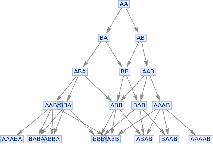
This graph can represent a quantum system with eigenstates represented by the vertices, where the initial state evolves over time. The property of common ancestry between two vertices can then be called entanglement. To represent entanglement relations for any given layer of the gaph, we can make a branchial graph:
In[]:=
Graph[ResourceFunction["MultiwaySystem"][{"A""B","B""AB"},"AA",4,"BranchialGraph"]]
Out[]=
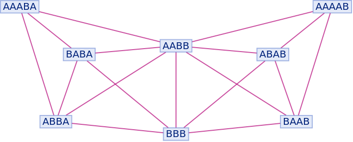
This represents the entanglement relations between these eigenstates: they are all connected, as they all share common ancestors.
To extend the Wolfram Model to a theory of measurement and observer effects, we can introduce the concept of observers as hypersurfaces. We have assumed a "motionless" observer, which is to say that there are, implicitly, horizontal foliations in our discussion above:
To extend the Wolfram Model to a theory of measurement and observer effects, we can introduce the concept of observers as hypersurfaces. We have assumed a "motionless" observer, which is to say that there are, implicitly, horizontal foliations in our discussion above:
In[]:=
Graph[ResourceFunction["MultiwaySystem"][{"A""B","B""AB"},"AA",4,"EvolutionGraph"],GraphLayout"LayeredDigraphEmbedding",Epilog{Red,Table[Line[{{-8,i},{8,i}}],{i,1/2,6+1/2}]}]
Out[]=
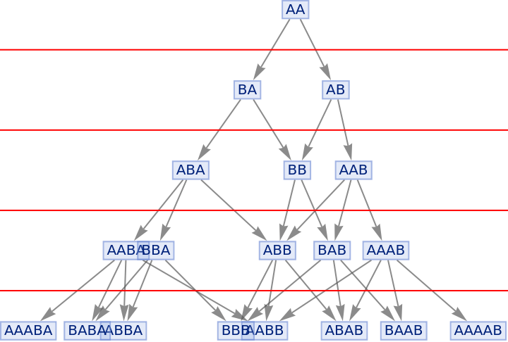
However, we can also imagine "boosted", or angled, foliations, just as in relativistic spacetime. Foliations are equivalence relations: all points on a foliation line are at the same time for the observer represented by the foliations. Sections created by equally spaced foliations constitute equal segments of time. An observer represented by a boosted foliation simply sees the quantum system as evolving "faster" on one side. Thus we can also consider a quantum system in a boosted foliation to be equivalent to a horizontally foliated quantum system with a different Hamiltonian.
Furthermore, the entanglement relations in a foliation can suggest equivalences, given by a Knuth-Bendix Completion Operator. Thus the number of entanglement relations also suggest the number of possible measured values, since by equivalence a superposition can be resolved into one state for an observer.
In this fleshed out conceptual framework, we can then suggest an analog to the conditions that give rise to Quantum Zeno Effect, a quantum system experiencing variable measurement density, in the Wolfram Model: the "trials" are given by equal-time-length foliations with variable numbers of entanglement relations or, equivalently, branchial edges. Here then is our initial question: can we show that the Wolfram Model gives rise to the quantum mechanical inverse law of time evolution speed with measurement density?
Predictions of the Wolfram Model
Predictions of the Wolfram Model
While many concepts in quantum mechanics can be translated consistently into the Wolfram framework, there are also some novel implications offered by the Wolfram Model. Chiefly, the Wolfram Model suggests a maximum entanglement rate in analogy with the maximum speed of light. This quantity emerges from the graphical representation of quantum mechanical states, in branchial space, and from our concept of observers as hypersurface foliations.
There is some basis to preliminarily expect a change in time evolution for different foliation: we can also understand the change in foliation as an altogether different Hamiltonian, and Hamiltonians have the same mathematical relationship as time to the quantum system's time evolution.
There is some basis to preliminarily expect a change in time evolution for different foliation: we can also understand the change in foliation as an altogether different Hamiltonian, and Hamiltonians have the same mathematical relationship as time to the quantum system's time evolution.
Computational Tools
Computational Tools
The first thing we would like to do is create foliations and associate with them a time, in arbitrary units, and number of branchial edges.
We will start with the simplest possible multiway graph, taking advantage of the straightFoliationLines function utilized in the technical introduction and this notebook, defined here. It creates foliation lines based on slope and on distance between lines, which will be left at 1.
We will start with the simplest possible multiway graph, taking advantage of the straightFoliationLines function utilized in the technical introduction and this notebook, defined here. It creates foliation lines based on slope and on distance between lines, which will be left at 1.
In[]:=
mwgraph[rule_,start_,iterations_,m_]:=Graph[ResourceFunction["MultiwaySystem"][rule,start,iterations,"EvolutionGraph"],GraphLayout"LayeredDigraphEmbedding",AspectRatio1/2,Epilog{straightFoliationLines[{1,0},{m,0},#&,{0,0},ResourceFunction["WolframPhysicsProjectStyleData"]["BranchialGraph","EdgeStyle"]]}] mwgraph[{"A""AB"},"AA",9,0.2]
Out[]=
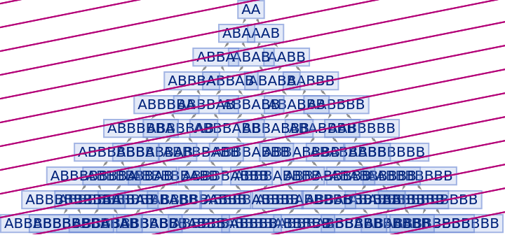
(For the sake of narrative, I am here sometimes chunking my functions into newer, more trivial ones so as to not write object-oriented manner, but the actual method utilized was to nest these small functions into one greater self-contained function. This is a superior method for running computational experiments as you can then nest the one function for any iterator of interest.) There are many possible approaches for identifying the eigenstates in each foliation, such as a biased Breadth-First Search. To this author, it was most intuitive to use the coordinates of the vertices and geometric analysis relative to the lines, although this is no doubt not as computationally optimized an approach.
In[]:=
findF[rule_,start_,iterations_,m_,coord_,F_]:=coord[[2]]>m*coord[[1]]+Round[-m*Max[GraphEmbedding[mwgraph[rule,start,iterations,m]]/.{x_,y_}x]]-0.5+F-1&&coord[[2]]<m*coord[[1]]+Round[-m*Max[GraphEmbedding[mwgraph[rule,start,iterations,m]]/.{x_,y_}x]]-0.5+FFoliationSets[rule_,start_,iterations_,m_]:=DeleteCases[_Integer]/@DeleteDuplicates/@Flatten/@GatherByTableDo[If[findF[m,GraphEmbedding[mwgraph[rule,start,iterations,m]][[n]],F],Return[F]],{F,∞}],Flatten[rule,start,iterations][[n]],{n,VertexCount[mwgraph[rule,start,iterations,m]]},FirstFoliationSets[{"A""AB"},"AA",9,0.2]
Out[]=
{{AA},{AAB,ABA},{AABB,ABAB,ABBA,ABBBA},{AABBB,ABABB,ABBAB,ABBBAB,ABBBBA},{AABBBB,ABABBBB,ABBABBB,ABBBABB,ABBBBABB,ABBBBBAB,ABBBBBBA},{ABABBB,ABBABB,ABBBBAB,ABBBBBA},{AABBBBB,ABBABBBB,ABBBABBB,ABBBBBABB,ABBBBBBAB,ABBBBBBBA,ABBBBBBBBA},{AABBBBBB,ABABBBBB,ABBABBBBB,ABBBABBBB,ABBBBABBB,ABBBBBABBB,ABBBBBBABB,ABBBBBBBAB,ABBBBBBBBAB,ABBBBBBBBBA},{AABBBBBBB,ABABBBBBB,ABBBABBBBB,ABBBBABBBB,ABBBBBBABBB,ABBBBBBBABB},{AABBBBBBBB,ABABBBBBBB,ABBABBBBBB,ABBBBABBBBB,ABBBBBABBBB},{AABBBBBBBBB,ABABBBBBBBB,ABBABBBBBBB,ABBBABBBBBB}}
Thus we can create sublists of the eigenstates in each foliation for any rule, initial state, number of iterations, and foliation slope.
It is easy enough to associate a time, since units are arbitrary: time can take the same value as the foliation level. Finally, we should be able to find the branchial edges for each foliation, as we demonstrate here for the 3rd, alongside its graph. It shows a much simpler branchial structure, i.e. much less entanglement, than the horizontal foliation.
It is easy enough to associate a time, since units are arbitrary: time can take the same value as the foliation level. Finally, we should be able to find the branchial edges for each foliation, as we demonstrate here for the 3rd, alongside its graph. It shows a much simpler branchial structure, i.e. much less entanglement, than the horizontal foliation.
In[]:=
Rest[Subgraph[ResourceFunction["MultiwaySystem"][{"A""AB"},VertexList[ResourceFunction["MultiwaySystem"][{"A""AB"},"AA",9,"StatesGraph"]],1,"BranchialGraph"],#]&/@{ Map[ToString,FoliationSets[{"A""AB"},"AA",9,m][[1]]], Map[ToString,FoliationSets[{"A""AB"},"AA",9,m][[3]]]}] BranchialEdge[rule_,start_,iterations_,slope_,FL_]:=EdgeCount[Rest[Subgraph[ResourceFunction["MultiwaySystem"][rule,VertexList[ResourceFunction["MultiwaySystem"][rule,start,iterations,"StatesGraph"]],1,"BranchialGraph"],#]&/@{0,Map[ToString,FoliationSets[rule,start,iterations,slope][[FL]]]}][[1]]] BranchialEdge[{"A""AB"},"AA",9,0.2,3]
Out[]=

Out[]=
2
Now we have most of the basic tools to begin doing data analysis. The last important consideration is how to compare horizontal and slanted foliations: we cannot simply relate the 6th segment to the 6th, but rather the slanted foliation must be compared only to a horizontal foliation of which it has reached all the members. The following expression, simplified by our sole consideration of positive-sloped foliations, does the job:
In[]:=
Do[If[MemberQ[FoliationSets["A""AB","AA",9,0.2][[c]],First[VertexList[ResourceFunction["MultiwaySystem"][{"A""AB"}, "AA", F, "BranchialGraph"]]]], Return[c]], {c,F, ∞}]
Verification of the Quantum Zeno Effect
Verification of the Quantum Zeno Effect
To begin our exploration of branchial edges, let's look at horizontal foliations for a few different rules.
In[]:=
ListPlot[{Labeled[Table[{Fol,EdgeCount[Graph[ResourceFunction["MultiwaySystem"][{"A""AB"},"AA",Fol,"BranchialGraph"]]]},{Fol,1,20}],"A -> AB"],Labeled[Table[{Fol,EdgeCount[Graph[ResourceFunction["MultiwaySystem"][{"A""B","B""AB"},"AA",Fol,"BranchialGraph"]]]},{Fol,1,5}],"A B, B -> AB"],Labeled[Table[{Fol,EdgeCount[Graph[ResourceFunction["MultiwaySystem"][{"A""AAB"},"A",Fol,"BranchialGraph"]]]},{Fol,1,5}],"A AAB"]},PlotLayout"Row",PlotMarkers{Automatic,Medium}]
These results are interesting and sensible: as time passes, each rule produces an increasing number of entangled eigenstates, whether linear or exponential; this is reminiscent of a spreading probability amplitude. We can also note that some rules (consider, for example, A -> B) go through a few iterations, and then stop with no further progression possible: there are operators that do this in quantum mechanics, too. For example, a repeated annihilation operator will eventually reach the vacuum state and quench.
We should here observe the challenge that, much like outside of the Wolfram Model, quantum computation grows exponentially complex at very small numbers. Thus we will be restricted to only a few iterations of simple rules, unless we do careful optimization.
Now, let's compare our simplest, linear-looking horizontal foliation rule with the same rule, but angled foliations. In general, the coordinate list relating time and number of branchial edges can be generate for the first 10 time units by the following code:
Let's plot the evolution of the number of entangled eigenstates with time, which is to say, the number of possible measurements. Note that there is a 0th state, which is simply the start of the rule (in our example, "AA"). Of course, the 0th state is not entangled with any other state.
(Note that slope 0.2 is the only one to extend to the 9th time step.) We find that for sloped foliations, the entanglements do not increase monotonically, or perhaps at all, with time. At earlier time values, the sloped foliations encapsulate the same eigenstates as the horizontal ones. As time passes, the sloped foliations capture significantly fewer entanglement relations than the horizontal foliations. The above graph could be interpreted as the effect of a changed Hamiltonian on the time evolution.
However, sloped foliations also represent greater observation density. By slope 0.75, we find that there is no increase in measurable state: time evolution is arrested, as we initially noted happens in the limit for the quantum Zeno effect. So, though this graphical formalism may be a useful mathematical tool to explain a variety of non-equivalent phenomena, here it seems we find a good representation of the Quantum Zeno Effect - and we find it emerging from an aspect of the Wolfram Model which is decidedly not a translation of current physics into a new graphical formalism, but rather a novel concept, not only of observation, but of observational relativity in quantum mechanics.
However, sloped foliations also represent greater observation density. By slope 0.75, we find that there is no increase in measurable state: time evolution is arrested, as we initially noted happens in the limit for the quantum Zeno effect. So, though this graphical formalism may be a useful mathematical tool to explain a variety of non-equivalent phenomena, here it seems we find a good representation of the Quantum Zeno Effect - and we find it emerging from an aspect of the Wolfram Model which is decidedly not a translation of current physics into a new graphical formalism, but rather a novel concept, not only of observation, but of observational relativity in quantum mechanics.
Concluding Remarks and Future Directions
Concluding Remarks and Future Directions
At the very least, the concepts of multiway and branchial graphs in the Wolfram Model constitute valuable structural tools for the description of quantum mechanics, and perhaps its suitability supports some much grander physical claim in reality, such as that our universe is fundamentally computational, discrete, or constructed from iteration of an elementary rule. In this project we have found yet another phenomenon that fits into the graphical formalism so well as to almost seem trivial. Future plans fall in three major categories.
First, the scope of this project was significantly hindered by the need for optimization. The lowest-hanging fruit would be to move from string substitution systems to a more efficient one; for example, one could easily use 0s and 1s instead of As and Bs, and store the composite bits as integers, as I have done in other quantum simulation projects. Then, the functions which were in this case written in as fast and physically intuitive a manner as possible given the time frame and the author's relative newness to the Wolfram Language. The geometric-inspection function for sorting , and in general agglomerated basic list comprehension functions should be replaced with more sophisticated and higher level frameworks. Nikolay Murzin has already written no doubt superior code to perform similar tasks. This optimization might allow for enough point-sampling for the establishment of a nonlinear relationship between the boosted and horizontal foliations, as well as the analysis of more complicated rules.
Next, it would also be very interesting to relate different types of quantum systems to different rules. While the wider goal of the Wolfram Model seems to be to find the one rule that describes our universe, in the quantum systems, various rules seem like they could best describe the different states, parameters, and operations that describe evolving quantum systems (e.g., spin, spin statistic, discrete location, position, momentum, number). This could be extended to establish a mapping between an experiment, such as ultracold atoms in optical lattices, and a Wolfram rule, as well as, with a bit more difficulty, a measurement and a foliation. Then, using past or future experimental data giving the dependence of the Zeno effect (survival amplitude) on various measurement quantities, we could move past the arbitrary time units of this analysis and perhaps erect the graphical modeling on real units of spacetime. Several experiments have established relationships between measurement parameters such as those of the imaging lasers. Wolfgang Ketterle and David Pritchard demonstrated a linear relationship between the lifetime of the initial state and the measurement density, and a trigonometric-exponential relationship between survival probability and number of measurements in a unit of time, asymptotically approaching 1.
Finally, it may be possible to extent these results for insight into the maximum entanglement rate by further graphical analysis along the lines of special relativity's Lorentzian algebra or Minkowski diagrams. While a very rough measurement exists in the Wolfram Model today, it would be very valuable to find a better scale for it, with implications for the elementary branchial length. This path of inquiry currently appears to be one of the most promising for experimental verification of the Wolfram Model.
Keywords
Keywords
◼
Quantum measurement
◼
Branchlike hypersurfaces
◼
Entanglement
Acknowledgment
Acknowledgment
I'd like to thank Jonathan Gorard, for his introduction to the quantum mechanical constructs in the Wolfram Model, both in our conversations and through his papers, physically, mathematically, graphically, and philosophically (usually all four at once). His attempts to clarify confusion by introducing more advanced mathematical terminology were cherished. I am also grateful for the help of Nikolay Murzin. I am equally inspired by Stephen Wolfram's willingness to ask questions and give advice, and beyond thankful for the time he gave to my project and to our shared interest in quantum measurement - his wiser intuition and emphasis shapes my own. Finally, many thanks to Danielle and Xerxes, who ensured that I received mentorship as schedules became hectic, and whose demeanor and insight brightened every School meeting.
References
References
◼
J. Gorard (2020). “Some Quantum Mechanical Properties of the Wolfram Model."
◼
Patil, Y. & Chakram, S. & Vengalattore, Mukund. (2014). "Quantum Control by Imaging : The Zeno effect in an ultracold lattice gas."
◼
Streed, E. & Mun, Jongchul & Boyd, Micah & Campbell, Gretchen & Medley, Patrick & Ketterle, Wolfgang & Pritchard, David. (2007). "Continuous and Pulsed Quantum Zeno Effect."