Suppose A is a d-by-d diagonal + rank1 matrix (DPR1).
We can compute statistics of in O(d) time, how can we compute statistics of in O(d) time?
Contour integrals to the rescue!
We can compute statistics of
-1
A
100000
A
Contour integrals to the rescue!
This post will show how the problem above connects to:
1. complex analysis
2. bird populations dynamics
3. neural network training
1. complex analysis
2. bird populations dynamics
3. neural network training
And will highlight contributions of Wolfram Language community.
In[]:=
Motivation
Motivation
Toy model: bird competition
Toy model: bird competition
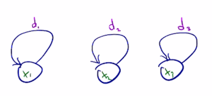
Consider the model of d=3 species on an island which grow according to per-species rates d1, d2, d3.
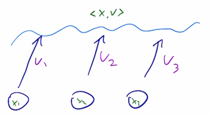
Additionally they pollute the environment at rates v1,v2,v3
And are affected by pollution proportionally to u1,u2,u3
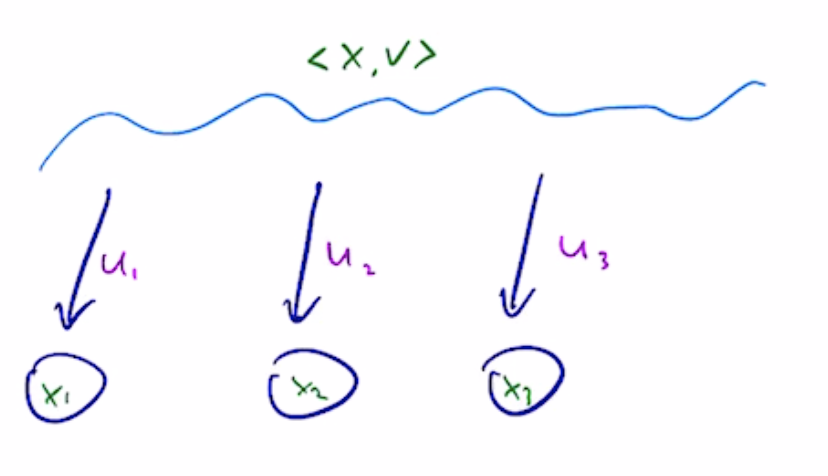
This is an instance of a mean-field model -- species interact with each other though a single shared factor.
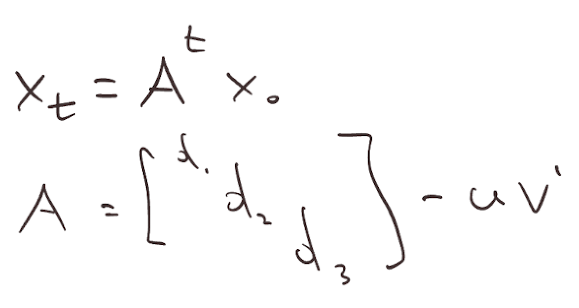
You could model their evolution by the following difference equation.
You could model their evolution by the following difference equation.

Alternatively, you can write it down in matrix form in terms of diagonal + rank1 matrix A
When A is symmetric, solution is written in terms of A eigenvectors.
Normally, this takes) operations, however, you can exploit DPR1 structure to do it in ) time.
Normally, this takes
O(
3
d
O(
2
d
Henrik Schumacher walks through an implementation of algorithm in Mathematica in this post and makes his implementation available at
- https://github.com/HenrikSchumacher/DPR1Eigensystem (url)
O()
2
d
- https://github.com/HenrikSchumacher/DPR1Eigensystem (url)
Neural Network Training
Neural Network Training
Neural networks take a long time to train, how do we make it faster?
A closely connected question is:
How long does a neural network take to train?
Under some simplifying assumptions, training a neural network takes at least as long at it takes for the following iteration to reach 0:
A closely connected question is:
How long does a neural network take to train?
Under some simplifying assumptions, training a neural network takes at least as long at it takes for the following iteration to reach 0:
e
r
e
r
e
r
Here x a zero-centered Gaussian variable with covariance eigenvalues h.
h corresponds to NTK eigenvalues of the Neural Network objective.
(Simplifying assumptions)
(Simplifying assumptions)
For Neural Networks, h corresponds to non-negative part of “NTK spectrum” or the “Hessian spectrum” and has empirically been observed to follow power-law decay, with p around 1.1
Algebraically, random linear recurrence like is hard. Finding the rate of decay is equivalent to the problem of finding Lyapunov exponent of a random matrix variable, intractable even for toy examples.
See
- Mathoverflow post.
- Section 3.3 of Matrix Concentration for Products paper
Numerically however, this recurrence appears easy in high dimensions. “Average trajectory” appears to be a good proxy for a “typical” trajectory. “Average” trajectory obeys a deterministic linear dynamical system.
Algebraically, random linear recurrence like
ee-x〈e,x〉
See
- Mathoverflow post.
- Section 3.3 of Matrix Concentration for Products paper
Numerically however, this recurrence appears easy in high dimensions. “Average trajectory” appears to be a good proxy for a “typical” trajectory. “Average” trajectory obeys a deterministic linear dynamical system.
Out[]=
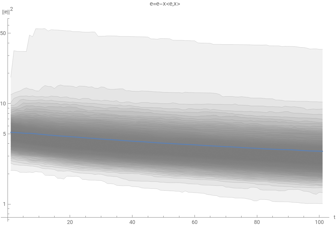

To study the average trajectory, use Wick’s theorem to get linear recurrence for . It’s a DPR1 linear system given by Equation 5 of Bordelon paper. In high dimensions, terms are insignificant, so we can use an even simpler recurrence for the average trajectory:
E[]
e
r
t
e
r
2
h
ee-2he+h〈e,h〉
Note the similarity of this update to bird population dynamics.
DPR1 SGD problem
DPR1 SGD problem
Restricting attention to DPR1 problem of neural network dynamics, we have the following linear recurrence We are interested to know L1 norm of e after t steps, which can be written as follows J(t) represents expected squared error after t steps of SGD on linear problem with eigenvalues h
ee-2he+h〈e,h〉
J(t)11
t
(I+A)
A-2diag(h)+h
t
h
How this DPR1 system maps to Neural Network training
How this DPR1 system maps to Neural Network training
For typical values of h (background here), J(t) is well approximated by matrix exponential
For typical values of h (background here), J(t) is well approximated by matrix exponential
J(t)1exp(tA)1
Out[]=
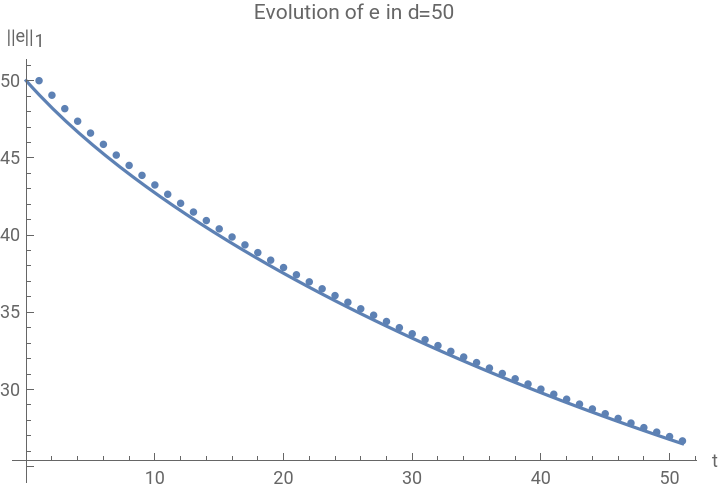


Under this approximation, we can obtain value of e after t steps by calling InverseLaplaceTransform on the resolvent of A, explained in Boyd’s autonomous linear systems slides:
et$=InverseLaplaceTransform[Inverse[s*ii-A],s,t].e0$;
In 10 dimensions, a random 2 dimensional projection shows that that “continuous” trajectory which relies on exp approximation is reasonably close to the original one.
Out[]=
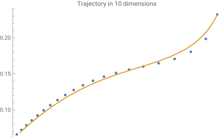

This recipe involves resolvent of A which is cheap due to Woodbury identity, which suggest a path to using DPR1 structure.
Solution from complex analysis
Solution from complex analysis
Now use two kinds of contours with built-in NIntegrate
Both methods are tractable because:
1. number of poles of f is small since rational approximation of small degree suffices
2. eigenvalues of A=-2diag(h)+hh can be read off diagonal of A, due to Gershgorin Circle Theorem.
1. number of poles of f is small since rational approximation of small degree suffices
2. eigenvalues of A=-2diag(h)+hh can be read off diagonal of A, due to Gershgorin Circle Theorem.
Examining the inner sum for d=3, we can see it’s a rational function of degree d, as a consequence of the Woodbury Matrix Identity.
We can thus avoid forming d-by-d matrix, and get tractable estimate of J by substituting expression analogous to the one above into one of two summations suggested by the resolvent method.
Community discussions
Community discussions
Continuous mean-field approximation
Continuous mean-field approximation
Simulation shows this approximation gives an upper bound for small d. Tight fit for large d.
Fast Gaussian number generation
Fast Gaussian number generation
Gaussian simulations above were bottlenecked by Gaussian number generation.
Discussion from Greg Hurst and Henrik Schumacher provided solutions on how to make this generation fast
- https://mathematica.stackexchange.com/questions/282210/speeding-up-gaussian-sampling (url)
On M2 MacBook Pros, GPU could potentially could make this generation 800 times faster. On older MacBook Pro’s, using SeedRandom[Method -> “MKL”] gives the most bang for the buck.
Dropping the rank1 term
Dropping the rank1 term
Suppose we drop the rank1 term to get a simpler update equation:
Ulrich Neumann, JimB show how to use Asymptotic to get an expression without Incomplete Gamma in the infinite d limit
https://mathematica.stackexchange.com/a/283913/217 (url)
https://mathematica.stackexchange.com/a/283913/217 (url)
Fast DPR1 computation using Zassenhaus formula
Fast DPR1 computation using Zassenhaus formula
Matrix Exponential of DPR1 matrix would be easy if we could exponentiate diagonal and rank1 terms separately.
Zassenhaus formula provides this.
I.M. provides implementation of Zassenhaus formula in this post:
https://mathematica.stackexchange.com/questions/282497/zassenhaus-formula-in-mathematica (url)
Zassenhaus formula provides this.
I.M. provides implementation of Zassenhaus formula in this post:
https://mathematica.stackexchange.com/questions/282497/zassenhaus-formula-in-mathematica (url)
Faster InverseLaplaceTransform
Faster InverseLaplaceTransform
Mariusz Iwaniuk made me aware of the Heavyside formula which can be used to obtain error after t steps much faster than built-in InverseLaplaceTransform.
https://mathematica.stackexchange.com/questions/282617/approximating-exponential-generating-function-egf-from-values-of-generating-fu/282625#282625 (url)
Meanwhile a problem with by Laplace Transforms due to bug in IntegrateChangeVariables got a workaround from Lacia
https://mathematica.stackexchange.com/questions/282080/is-this-a-bug-in-integratechangevariables (url)
Wick’s Theorem
Wick’s Theorem
Gaussian recurrence in low dimensions
Gaussian recurrence in low dimensions
However, we can find the threshold numerically, JimB and Michael E2 provide code to compute the relevant integral:
https://mathematica.stackexchange.com/questions/272484/speeding-up-computation-of-gaussian-integral (url)
Related materials for obtaining low-d convergence threshold are summarized here
https://mathematica.stackexchange.com/questions/272484/speeding-up-computation-of-gaussian-integral (url)
Related materials for obtaining low-d convergence threshold are summarized here
CITE THIS NOTEBOOK
CITE THIS NOTEBOOK
Neural networks, bird populations, complex analysis and DPR1 matrices
by Yaroslav Bulatov
Wolfram Community, STAFF PICKS, April 20 2023
https://community.wolfram.com/groups/-/m/t/2902848
by Yaroslav Bulatov
Wolfram Community, STAFF PICKS, April 20 2023
https://community.wolfram.com/groups/-/m/t/2902848