WOLFRAM NOTEBOOK

In[]:=
CompoundExpression[
]
deploy
Thu 4 May 2023 01:40:19

Power-law decay of Velikanov, Berthier, Zeke Xie

Summary:
- Grosse observed
-1
i
decay
by looking at KFAC factors of Gauss-Newton matrix
- Zeke Xie observes
-1.1
i
decayofNTKeigenvalues.TheydiscardtopKeigenvalueswhereK=numberofclasses.

- Velikanov observed
-1.3
i
decay and obtains power law decay of loss by finding generating function of the loss and applying Tauberian theorem. (TODO, get explicit formula for their approach)
- Berthier gives simulation on Gaussian linear least squares with
-1.4
i
decay and obtains
-0.29
s
decay in loss* by taking dimensionality to infinity
*Technically Berthier gives decay in error given non-uniform starting distribution, but it’s equivalent to decay in loss with isotropic starting distribution

top level section: Diagonal + rank1

Grosse, “Which Algorithmic Choices Matter at Which Batch Sizes?” https://arxiv.org/abs/1907.04164
(verified on CIFAR spectrum experiments here)

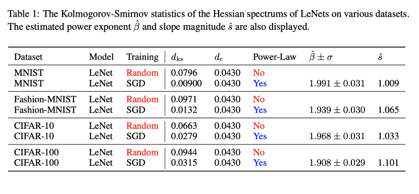
Zeke Xie “On the Power-Law Hessian Spectrums in Deep Learning”
https://arxiv.org/abs/2201.13011

Velikanov “A view of mini-batch SGD via generating functions: conditions of convergence, phase transitions, benefit from negative momenta”
https://arxiv.org/abs/2206.11124

“Tight Nonparametric Convergence Rates for Stochastic Gradient Descent under the Noiseless Linear Model”
https://arxiv.org/abs/2006.08212

Other notebooks:
- https://www.wolframcloud.com/obj/yaroslavvb/nn-linear/berthier-formulas.nb

Section 3.3 of Berthier’s Tight Nonparametric Convergence Rates

In Gaussian setting, e(s) can be computed exactly using Eq 5 in Bordelon’s “structured features” paper as follows

Code

In[]:=
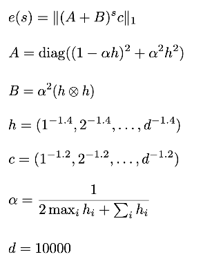
d=10000;(*dimensions*)numSteps=d;β=1.4;(*spectrumdecay*)δ=1.2;(*initialerrordecay*)h=Table[
-β
i
,{i,1,d}];(*Covariancespectrum*)c=Table[
-δ
i
,{i,1,d}];(*initialerrorvector*)c=c/Total[c];SF=StringForm;α=
1
Total[h]+2Max[h]
;(*stepsize,1/2ofmaximalcontractiveforerrorcovinSchatten-1norm*)(*diag+rank-1update.ComesfromEq.5inBordelon"structured features",specializedtoC=diag(c)*)step[c_]:=(
2
(1-αh)
+
2
α
2
h
)c+
2
α
hTotal[hc];cs=NestList[step,c,numSteps];observedVals=Total/@cs;stepVals=Table[s,{s,0,numSteps}];predictedVals=
-0.29
(#+1)
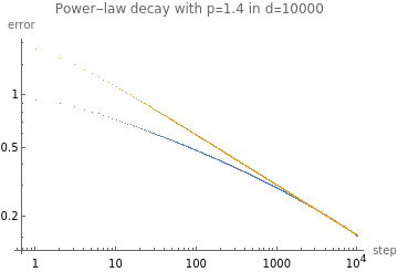
&/@stepVals;nudge=2.25;observed={stepVals,observedVals};predicted={stepVals,nudge*predictedVals};ListLogLogPlot[{observed,predicted},PlotRange->All,PlotLegends->{"observed",SF["``*
-0.29
s
",nudge]},AxesLabel->{"step","error"},PlotLabel->SF["Power-law decay with p=`` in d=``",β,d]]
Out[]=
observed
2.25*
-0.29
s

What power-law constant to use?

- “ON THE POWER-LAW HESSIAN SPECTRUMS IN DEEP LEARNING” https://arxiv.org/pdf/2201.13011.pdf
(*MNIST*)β=1.939;p=
1
β-1
Out[]=
1.06496
In[]:=
(*CIFAR*)β=1.908;p=
1
β-1
Out[]=
1.10132
In[]:=
p=1.4d=20000;(*dimensions*)numSteps=d/2;β=p;(*spectrumdecay*)δ=0;(*initialerrordecay*)h=Table[
-β
i
,{i,1,d}];(*Covariancespectrum*)c=Table[
-δ
i
,{i,1,d}];(*initialerrorvector*)c=c/Total[c];SF=StringForm;α=
1
Total[h]+2Max[h]
;(*stepsize,1/2ofmaximalcontractiveforerrorcovinSchatten-1norm*)(*diag+rank-1update.ComesfromEq.5inBordelon"structured features",specializedtoC=diag(c)*)step[c_]:=(
2
(1-αh)
+
2
α
2
h
)c+
2
α
hTotal[hc];cs=NestList[step,c,numSteps];observedVals=h.#&/@cs;stepVals=Table[s,{s,0,numSteps}];(*predictedVals=
-0.29
(#+1)
&/@stepVals;*)predictedVals=0;observedData={stepVals,observedVals};ListLogLogPlot[{observedData},PlotRange->All,PlotLegends->{"observed",},AxesLabel->{"step","error"},PlotLabel->SF["Power-law decay with p=`` in d=``",p,d]]logStepVals=Rest[Log/@stepVals];logObservedVals=Rest[Log/@observedVals];data={logStepVals,logObservedVals};dataToFit=data[[Floor[Length[data]/2];;]];(*usesecondhalfforfitting*)lm=Normal@LinearModelFit[dataToFit,x,x];logPedictedPlot=Plot[lm,{x,Min[logStepVals],Max[logStepVals]},PlotLabel->"Predicted"];logObservedPlot=ListPlot[Log@Rest@observedData];(*Show[logPedictedPlot,logObservedPlot,PlotLabel->"logs"]*)linearFit=Exp[lm/.x->Log[s]];berthierZ=3103.527039817376`;berthierFit=
-0.29
s
/berthierZ;predictedPlot=Plot[{None,linearFit,berthierFit},{s,1,numSteps},ScalingFunctions->{"Log","Log"},PlotLegends->{"",SF["`` (empirical)",linearFit],SF["``(berthier)",berthierFit]}];observedPlot=ListPlot[Rest@observedData,ScalingFunctions->{"Log","Log"}];Show[predictedPlot,observedPlot,PlotLabel->"loss of Gaussian SGD with `` decay"]

What power law does deterministic GD follow?

Can get explicit formula by taking Laplace transform in terms of Exponential integrals
Wolfram Cloud

You are using a browser not supported by the Wolfram Cloud

Supported browsers include recent versions of Chrome, Edge, Firefox and Safari.


I understand and wish to continue anyway »

You are using a browser not supported by the Wolfram Cloud. Supported browsers include recent versions of Chrome, Edge, Firefox and Safari.