Preparing a specific quantum state is a basic step in almost any quantum computation, and doing it with as few operations as possible matters, since every gate adds error on real hardware. This project studies how to prepare arbitrary two-qubit states using a structure-aware approach. Rather than applying a single general method to every state, I develop a method for synthesizing quantum circuits that prepare arbitrary pure quantum states by exploiting their underlying structure. These circuits achieve near-perfect fidelity using the theoretical minimum number of entangling gates, matching the bounds established by earlier research. Compared with a general-purpose variational method that ignores structure, they use fewer gates and run substantially faster because the circuit is computed directly rather than found by search. This is among the first structure-aware two-qubit state preparations built in the Wolfram Quantum Framework, and I also explore how the approach extends to three qubits and beyond.
Introduction
Introduction
One of the most challenging components of quantum computing is the complexity of circuits with multiple qubits. A good way to conceptualize qubits is through the analogy of a coin. In classical machines, a bit can be thought of as a coin lying flat with either heads or tails (a 1 or a 0). However, in quantum computing, the coin is spinning, acting as a blur that represents both states at the same time until it is measured (think of this as stopping the spinning coin to see its face). This principle is known as superposition, and in this analogy, because this coin lies in these conditional states, I can assign probabilistic amplitudes to each face. While an ideal coin flip yields a 50/50 chance of heads or tails, quantum computers allow us to adjust these odds by biasing the spin to favor certain outcomes using complex numbers. These amplitudes are more than simple probabilities, as they also carry a property called phase, which has no classical counterpart and becomes important once qubits begin to interact with one another.
Before a quantum computer can perform any useful task, it must first be placed into a specific state to make the algorithm useful. This task is known as state preparation, and it is the focus of my work. Every computation begins from a simple, known starting point, and I must transform that starting point into a desired target state using a sequence of operations called a quantum circuit. A circuit is built from quantum gates, which are the basic operations that rotate, flip, or entangle qubits, much like logic gates manipulate bits in a classical computer. The challenge is that many different circuits can reach the same target state, yet they are not equally good. Some use far more gates than necessary, and on real hardware, every additional gate incurs a cost and increases the likelihood of errors. Finding the shortest and simplest circuit for a given state is therefore not only a theoretical curiosity but a practical necessity for making quantum computers reliable.
In this project, I worked on quantum circuit synthesis where the goal is to reach a given end state, progressing from single-qubit to multi-qubit cases. Rather than treating every state the same way, my approach is to first examine the target state' s structure and then choose a preparation method suited to it. Some states are simple and require very little to build, while others are far more complex and demand more careful treatment. By recognizing these differences, I can prepare each state efficiently and reliably, avoiding unnecessary operations wherever possible. I develop this idea gradually, beginning with single-qubit states to establish the core concepts, then extending to the full range of two-qubit states, including the entangled ones that represent the hardest and most interesting case. Although my focus is on two qubits, the principles I develop here form the foundation for tackling larger, more demanding systems where efficient state preparation matters most.
The 1 Qubit Case
The 1 Qubit Case
Load the Wolfram Quantum Framework :
PacletInstall["Wolfram/QuantumFramework"]Needs["Wolfram`QuantumFramework`"]
I start with 1 qubit circuits, and the method to move these circuits to their end state is fairly straightforward. Principles such as entanglement do not apply to them, as they have no other qubits to get entangled with.
A single qubit circuit’s state can be imagined as some point on the Bloch Sphere, and it must move to another point:
In[]:=
qs=QuantumState["1"]
Out[]=
|1〉
In[]:=
qs["BlochPlot",ImageSize->Small]
Out[]=

For clarity, the Bloch Sphere representation of this example points to where the state is currently, and can point to anywhere on this sphere depending on where the state is, this example points to
|0〉.
Applying rotations to move its position :
In[]:=
qc0=QuantumCircuitOperator[{"1","RX"[π/2]}];qc0["Diagram"]
Out[]=
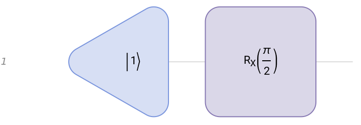
Rotate by an angle both for its longitude and latitude :
In[]:=
qc0[]
Out[]=
-|0〉+|1〉
2
1
2
In[]:=
qc0[]["BlochPlot",ImageSize->Small]
Out[]=

In general, any single qubit is prepared using two rotations: starting from the state, a rotation about the Y axis tilts the qubit by an adjustable angle θ, and a rotation about the Z axis sets its phase by an angle φ. Together these two rotations can reach any single qubit state, and the angles θ and φ are the dials I adjust to select which state.
|0〉
Build a parametrized circuit, leaving the two angles as free parameters:
In[]:=
circuit1=QuantumCircuitOperator[{"0","RY"[θ]->1,"RZ"[ϕ]->1},"Parameters"->{θ,ϕ}];circuit1["Diagram"]
Out[]=
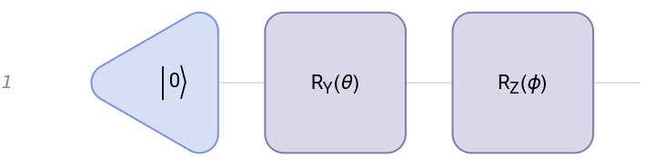
The diagram shows the two rotation gates in sequence. This is the general template for preparing any single qubit state, differing only in the angle values chosen.
Compute the probability of each measurement outcome as a function of the angles:
In[]:=
probs=ComplexExpand/@circuit1[]["Probabilities"]
Out[]=
0+,1+
2
Cos
θ
2
2
Cos
θ
2
2
Sin
θ
2
2
Sin
θ
2
2
Cos
θ
2
2
Sin
θ
2
These expressions show that the measurement probabilities depend directly on the angle θ, shifting smoothly as it changes.
Plot these probabilities as θ sIeps through a full rotation :
In[]:=
PlotEvaluate@Values[probs],{θ,0,2π},
Out[]=
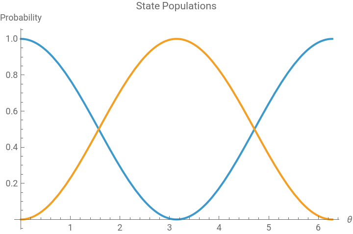


The curves show how the rotation controls the qubit. At it stays in ; as θ increases, probability flows to the outcome, passing through an even fifty-fifty split at , the equator of the Bloch sphere, and reaching | 1 ⟩ at .
θ=0
|0〉
|1〉
θ=π/2
θ=π/2
By choosing the angle, I set the exact odds of each outcome. This is the spinning coin idea made precise. The next question follows naturally :
Given a target state, how do I find the angles that produce it?
Extract the globe coordinates out of the target state :
In[]:=
angles1=QuantumState["+"]["BlochSphericalCoordinates"][[2;;]]
Out[]=
,0
π
2
Here, I take a target state and read its two global angles θ and ϕ out of its amplitudes. Notice how the angles align with the point on the sphere above. Next, I then turn these angles into a runnable circuit.
Start at and apply the gates, tilting then turning on qubit 1:
|0〉
In[]:=
qc1=circuit1[AssociationThread[{θ,ϕ}->angles1]];qc1["Diagram"]
Out[]=
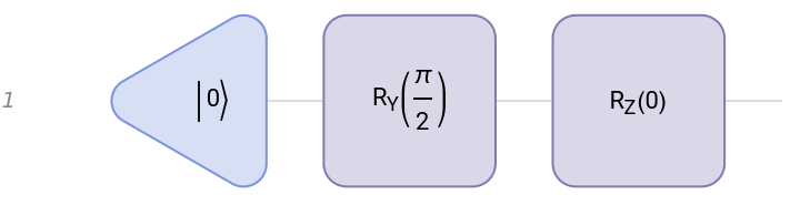
To verify that this circuit gets to the desired end state, run the circuit and measure its fidelity(how close it gets to the target state):
In[]:=
QuantumSimilarity[qc1[],QuantumState["+"]]
Out[]=
1
Since there is no entanglement involved, it is virtually guaranteed that I can reach a near perfect 1.0 fidelity(meaning it exactly matched the target state) testing across n random target states.
The 2 Qubit Case
The 2 Qubit Case
The real difficulty begins when I combine multiple qubits. A single qubit is relatively simple to describe on its own, but when two or more qubits interact, they can become entangled, meaning their outcomes are linked so that one cannot be fully described without the other. In an entangled state, the system behaves as a single connected whole rather than as a collection of independent parts. This connection has no classical equivalent and is a major part of what gives quantum computers their power, as it allows them to represent and process information in ways classical machines cannot. At the same time, it is what makes multiple-qubit systems so much harder to work with, because the number of possible states and the effort required to control them grow rapidly as more qubits are added.
4 example states :
In[]:=
QuantumState["RandomPure"[2]]
Symbolically :
α|00〉+β|01〉+χ|10〉+δ|11〉
Numerically :
Out[]=
(-0.387365-0.371627)|00〉+(-0.258761+0.223382)|01〉+(-0.601981-0.289329)|10〉+(0.191832+0.334803)|11〉
The Bloch Sphere is no longer a valid model, as it cannot represent two qubit circuits because the state space of two qubits requires a 4-dimensional complex vector space. A single qubit operates in a 2-dimensional space, which maps perfectly to the 2D surface of a 3-sphere.
Two qubits operate on a = 4-dimensional Hilbert space:
2
2
In[]:=
QuantumState["RandomPure"[2]]["Dimension"]
Out[]=
4
Additionally, two-qubit systems can form entangled states, like Bell states:
In[]:=
QuantumState["Bell"]
Out[]=
1
2
1
2
In this case qubits have non-local correlations. Entanglement is a relationship betIen qubits, and it is impossible to visualize this connection on individual Bloch spheres.
Alongside the current gates that, in the later more complicated situations the CNOT gate will be used:
In[]:=
QuantumCircuitOperator[{"CNOT"}]["Diagram",ImageSize->Small]
Out[]=
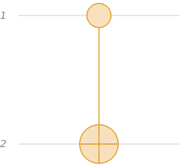
CNOT is a gate that simply put links two qubits together, putting them in an entangled state to allow rotations to be applied to both at once, and its used when the target state is entangled. Before I tackle this, I first start simpler with the basis 2-qubit cases.
Basis States
Basis States
To prepare a basis state, I read the amplitude list to find which basis state the input is, express that as two bits, and apply an X gate to each qubit whose bit is.
This shows where in the state string there is 1:
The result is a circuit that uses at most two gates and never requires a CNOT, because a basis state contains no entanglement to build:
Separable States
Separable States
A separable state is defined as two independent qubits placed side by side, meaning they carry no entanglement. Because the qubits are independent, the state can be split into a separate piece for each one, and each piece can be prepared entirely on its own.
Applying the RY and RZ gates to each qubit independently reproduces the target state exactly .
Formulaic Representation
Build it up one step at a time:
Compute both qubits Bloch coordinates as {r, θ, φ}:
These angles are exactly what the rotations in the circuit will use:
The circuit applies an RY and RZ rotation to each qubit using the angles just found, and crucially, the two qubits are never connected.
There is no CNOT gate, because a separable state has no entanglement to create:
The state was prepared using only independent single qubit rotations, exactly as the separable structure allows. Because the qubits are prepared independently and never linked, the circuit contains no CNOT gate, exactly as a separable state requires.
Entangled States
Entangled States
I now arrive at the hardest and most important case. The basis and separable states that came before did not require a CNOT gate, because neither contained any entanglement. Their qubits could always be prepared independently, one at a time, and combined without ever linking them. An entangled state breaks this entirely, because its qubits cannot be described separately, and no amount of independent single-qubit preparation can ever produce the connection between them.
Verify how “entangled” is a quantum state computing the concurrence(a measure of entanglement between two qubits):
If the Concurrence is greater than 0, the state is entangled:
In order to build an entangled state, I need a gate that acts on both qubits at once and ties them together, so I use CNOT. A CNOT, short for controlled NOT, takes two qubits and uses one to decide the fate of the other.
One qubit acts as the control and the other as the target, and the rule is simple: if the control qubit is 1, the target qubit is flipped, and if the control is 0, the target is left alone:
On its own this sounds like an ordinary conditional operation, but when the control qubit is in a superposition, the effect is profound. The CNOT links the two qubits so that their outcomes become tied to one another, producing precisely the correlations that define entanglement.
The perfect example for an entangled state is the Bell State:
Compute the Concurrence:
The challenge, however, is not simply knowing that I need a CNOT. It is knowing exactly how to build a specific entangled state: which rotations to apply, how strong to make them, and how to arrange them around the CNOT so that the final result matches the target I am given.
Schmidt Decomposition
Schmidt Decomposition
An entangled state is described by four complex amplitudes with intricate relationships between them, and it is far from obvious how to translate those four numbers into a concrete sequence of gates. To do this, I need a way to see past the tangled surface of the state and expose the underlying structure of its entanglement.
The tool that accomplishes this is the Schmidt decomposition:
The Schmidt decomposition states that any two-qubit state, no matter how complicated it appears, can be rewritten as a combination of just two matched pairs of single-qubit states, which is an incredible simplification. A general two-qubit state seems to involve four independent amplitudes tangled together, but the Schmidt decomposition shows that beneath this apparent complexity, the state has a much simpler skeleton.
Weights for each of the qubits by generating a random 2 qubit Schmidt basis quantum state:
There exists a special basis for each qubit, chosen specifically for that state, in which the entanglement collapses into its simplest possible description: two terms, each pairing one basis state of the first qubit with one basis state of the second, and each weighted by a number:
These two weights, called the Schmidt coefficients, are at the heart of the decomposition because they measure exactly how much entanglement the state contains. Consider the two extremes: if one coefficient is one and the other is zero, then only a single term survives, the state reduces to a single pair of single-qubit states, and there is no entanglement at all.
The following shows a state with coefficients zero and one:
In the case the state is separable, and I have returned to the previous case entirely. If instead the two coefficients are equal, the two terms contribute with equal weight, and the state is maximally entangled, meaning the two qubits are as tightly connected as possible.
Maximally entangled Bell’s Phi Minus state:
Every entangled state lies somewhere along the spectrum between these two extremes, and the Schmidt coefficients pinpoint precisely where it falls. A state with coefficients close to one and zero is only weakly entangled, while a state with nearly equal coefficients is strongly entangled.
What makes this so useful is that it converts an impossibly tangled description into an organized one that I can act on. Before the decomposition, I had four amplitudes with no obvious meaning. After it, I have two clear pieces of information: a precise measure of how much entanglement to create, given by the Schmidt coefficients, and a precise specification of the bases each qubit must end up in, given by the single-qubit states in each pair.
The Schmidt decomposition has taken a problem that looked extremely challenging and split it into two manageable parts, each of which maps directly onto something a circuit can do. With the state reorganized in this way, the circuit follows a clear three-part structure, and each part corresponds to one piece of the Schmidt decomposition.
The first part sets up the qubits for the desired entanglement. A single rotation is applied to the first qubit, with an angle calculated directly from the Schmidt coefficients. This rotation sets the balance between the two Schmidt terms, and by choosing the angle correctly, I produce exactly the amount of entanglement the target state requires. At this stage, the qubits are prepared but not yet linked. The second part performs the linking and the actual entanglement. A single CNOT gate is applied, spreading the entanglement across both qubits and entangling their outcomes. The third part sets the final form. Two single-qubit operations, one on each qubit, rotate the qubits out of the special Schmidt basis and into the actual basis that the target state uses. These operations do not affect the amount of entanglement, which was already fixed by the first two parts. Instead, they orient the entangled pair correctly, placing it in its precise final configuration so that it matches the target exactly.
The following function implements this three part construction, taking any entangled two qubit state and building its circuit directly:
The function follows the three parts in order. It computes the Schmidt decomposition of the target and reads off its coefficients, using the first coefficient to set the entangling rotation angle. It then applies that rotation, followed by a single CNOT to create the entanglement, and finally the two basis rotations that turn the pair into its target configuration. The whole circuit is determined by the structure of the state and uses exactly one CNOT.
Applying it to a random entangled state confirms that it reproduces the target exactly :
With the entangled case solved, I have now covered all types of two-qubit states. Basis states, separable states, and entangled states can each be prepared exactly, and in each case, the circuit was built using the same strategy: examine the structure of the target and use that structure to construct the exact circuit directly. This approach is powerful, but it depends entirely on the ability to recognize and exploit a state’s structure. It is worth asking what happens when I set that ability aside. Suppose I were handed a state and wanted a single method that could prepare it without analyzing its structure at all, treating every state the same way. Such a general-purpose method serves two important roles. It serves as a universal fallback, preparing any state regardless of its form, and as a benchmark, revealing what state preparation costs when no structural insight is used. By comparing the structure-aware methods against it, I can measure exactly what is gained by recognizing a state’s structure. For this general approach, I turn to the Hardware Efficient Ansatz.
Hardware Efficient Ansatz Layout
Hardware Efficient Ansatz Layout
The Hardware Efficient Ansatz is a fixed circuit layout, a set arrangement of gates (operations that change qubits) whose structure stays the same, but whose individual gates have adjustable settings. It is built from two kinds of gates. The first are single-qubit rotations, which turn a qubit by an angle I can choose, like a dial set to any value. The second is the CNOT gate, which acts on two qubits at once and links them together, so that the state of one depends on the other. This linking is what creates entanglement, the very connection that could not be represented on individual Bloch spheres. Because single-qubit rotations act on each qubit independently, they can never produce this connection on their own; the CNOT is the gate that manufactures the entanglement a two-qubit target may require so that a rotation acts on both at once. The layout works in three stages. Every circuit begins with both qubits unentangled, in the state |00⟩.
In the example below, I am attaching the diagram of the quantum circuit at each stage, along with its values, to show how each stage transforms it, both visually and numerically.
First, a layer of rotations moves each qubit independently:
Then a CNOT links the two qubits, creating entanglement:
Finally, a second layer of rotations adjusts the now-entangled pair into its final configuration:
Below is the complete HEA for this circuit. It follows these three steps and returns the final output identical to the state after the third step above:
By adjusting the rotation angles alone, the same fixed layout can be tuned to yield many two-qubit states, both entangled and unentangled. To prepare a specific target, I begin with arbitrary angle settings and adjust them, repeatedly comparing the circuit’ s output to the state I want, until the two match. It is indeed hardware-efficient because it uses only rotations and CNOT gates that real quantum computers can perform reliably, rather than idealized operations that would be difficult or expensive to implement on actual hardware. Earlier, general approaches to state preparation often required circuits with many layers, which grew rapidly with system size, making them slow to optimize and costly to run. HEA keeps the layout compact enough to use only a few gates while reaching many different 2-qubit states. It was the focus for the first stage of reaching target states in 2-qubit circuits. The implementation of the HEA was a general-purpose fallback for any two-qubit target, used when no analytic specialist applies (i.e., entangled states).
Symbolic Representation
Symbolic Representation
The ansatz is a fixed circuit layout with eight adjustable angles. Because most two-qubit states can be reached by some setting of these eight angles, this one fixed layout is universal:
Visualize the 6 gates:
The resulting state has weight on all four basis states with complex amplitudes, confirming it is a genuine, arbitrary target rather than a simple or special case.
This is the state the optimizer will now try to reproduce by tuning the six angles of the ansatz :
A symbolic representation of all the possibilities of states generated by the circuit :
With the target chosen, preparing it becomes an optimization problem : find the six angles that make the ansatz output match the target as closely as possible. To measure the match, we define the fidelity, the squared overlap between the state the ansatz produces and the target. It equals one for a perfect match and less than one otherwise .
Use NMaximize to search for the angles that maximize it, recording the fidelity at each step so the search can be visualized afterward:
The optimizer succeeds, returning a fidelity of one along with the six angles that achieve it. These angles define the rotations needed to prepare the target state. Unlike the analytic specialists, which compute their circuit directly from the state' s structure, the ansatz arrives at this answer through search, adjusting the angles repeatedly until the output matches. The fidelity values recorded at each step, captured during the search, let us see how that convergence unfolded.
Visualizations
Visualizations
The curve shows the ansatz converging on its target. It begins far from the goal, at a fidelity of about 0.2, and climbs steadily as the optimizer improves the angles, until it reaches a fidelity of one, a perfect match. The staircase pattern is characteristic of the search : the optimizer settles briefly on a set of angles, then discovers a direction that improves them, producing a jump. This is the defining behavior of a variational method. Rather than computing the circuit directly, it feels its way toward the target through many small adjustments, and the many steps required stand in clear contrast to the analytic specialists, which arrive at their answer in a single calculation. Notice that in this test it takes 104 steps to reach a perfect fidelity, one of the main reasons HEA runs slower and is more expensive due to its lack of structure-aware methodology.
To see the optimization at work, we visualize the cost landscape. Since the ansatz has six angles but a plot can show only two, we vary two of them while fixing the rest at their optimal values, giving a two dimensional slice through the search space.
The color shows the fidelity at each point, with dark regions marking low cost:
The optimizer begins in a dark low cost region and works its way toward the light colored center where the circuit reproduces the target.
The same landscape can be viewed as three dimensional terrain, which shows more vividly how the optimizer ascends. The height of the surface is the fidelity so the search is a process of finding the highest point in a mountainous landscape :
Viewed as terrain, the goal of the optimization is quite intuitive: reach the top of the hill, where fidelity is one and the target is perfectly prepared. The optimizer climbs up from the low ground it started on, following the slope toward the local maximum. This is the geometric picture of a variational search, and it stands in contrast to the analytic specialists, which compute the location of the valley floor directly rather than descending into it.
Future Goals: Exploring 3 Qubits
Future Goals: Exploring 3 Qubits
The methods developed here handle the full range of two qubit states, and they point naturally toward a larger goal : extending the same structure aware philosophy to three qubits and beyond. The guiding principle remains unchanged: given a state, recognize its structure and let that structure determine the most efficient circuit. A three qubit state is described by eight complex amplitudes, one for each of its eight basis states, twice as many as the four that describe a two qubit state. This doubling, together with the richer entanglement it allows, is what makes three qubits a substantially harder problem.
The possible states of a 3 qubit circuit :
With this general form in mind, we can see how specific structured states arise as special cases with most of these amplitudes set to zero.
Among three qubit states, two special kinds stand out, and they turn out to be fundamentally different. Dür, Vidal, and Cirac proved that genuine three qubit entanglement splits into two distinct classes, named after their most famous examples : the GHZ state and the W state. These two classes cannot be transformed into one another by any operation acting on the qubits individually, which means they represent two separate kinds of entanglement, each requiring its own approach to prepare.
The GHZ state concentrates all of its weight on just two of the eight basis states:
The W state instead spreads its weight across three basis states, each with a single qubit excited:
Notice the contrast with the general form. Where an arbitrary three qubit state carries eight independent amplitudes, the GHZ state uses only two and the W state only three. This sparsity is the structure a preparation method exploits : rather than solving for all eight amplitudes, it recognizes that most are zero and builds a far simpler circuit for each case.
The distinction between the two classes becomes even clearer when we look at their measurement probabilities directly:
The GHZ state places equal weight on all zeros and all ones, with nothing in between, capturing a correlation that is all or nothing across the whole system. The W state spreads its weight evenly across the three states with a single excitation, reflecting a connection shared among the qubits rather than concentrated at the extremes.
These structures can also be seen geometrically. If we place the eight basis states at the corners of a cube, connecting states that differ by a single qubit, and size each corner by its amplitude, the two classes take on visibly different shapes:
Each corner of the cube is one of the eight basis states, and the edges connect states differing by a single qubit. The GHZ state appears as two large spheres at opposite corners, its weight concentrated on all zeros and all ones. The W state appears as three equal spheres sharing a single face, its weight spread across the states with one excitation. The geometry makes the structural difference between the two classes immediately visible.
A full three qubit method would follow the same classify and construct strategy used throughout this project, extended to more cases. It would first determine a state' s structure, then dispatch it to a specialized circuit:
Basis and separable states extend directly and need no entangling gates. Biseparable states, where one qubit is independent while the other two are entangled, reduce to the two qubit entangled circuit already developed here, applied to the correlated pair. The tripartite states, GHZ and W, require their own dedicated constructions using two entangling gates. This mirrors exactly the logic used for two qubits, with the two qubit specialists becoming building blocks for the three qubit case.
Extending to three qubits also strengthens the case for structure aware methods, because the cost of ignoring structure grows rapidly.
The general purpose method uses a fixed number of CNOT gates given by the formula two to the power n plus two, minus four n, minus four, a number that escalates quickly with each added qubit:
The general purpose method uses a fixed number of CNOT gates given by the formula two to the power n plus two, minus four n, minus four, a number that escalates quickly with each added qubit:
The general purpose CNOT count rises steeply : none for a single qubit, four for two, sixteen for three, and forty four for four. A structure aware method, by contrast, uses only the entangling gates a state genuinely requires, often far fewer. As systems grow, this gap widens dramatically, which means the deeper a system' s structure, the more there is to gain by recognizing it.
The Broader Goal
The Broader Goal
Beyond these structured families lies the fully general three-qubit state. Recent work by Lee and Kim provides a complete classification of three-qubit pure states into five types, each with an explicit circuit template derived from the Schmidt decomposition across a bipartition. Implementing this full classification within the Wolfram Quantum Framework and verifying that its circuits achieve the known minimum gate counts is the natural continuation of this work. Several other directions also follow: improving the variational fallback to reduce its search time, testing these circuits on real quantum hardware, where lower CNOT counts should yield measurably higher fidelity, and extending the classification to mixed states for more realistic, noisy settings. The broader goal this project builds toward is a single system that, given any state of any size, recognizes its structure and produces the most efficient circuit possible, turning to search only when no structure can be found.
Conclusion
Conclusion
This project set out to prepare arbitrary two-qubit states using circuits that when evaluated, match them exactly. It succeeded by taking a structure-aware approach. Rather than applying a single general method to every state, I first examined each target’s structure and used it to construct a tailored circuit. Basis states were prepared with simple bit flips, separable states with independent single-qubit rotations read directly from the Bloch sphere, and entangled states with a Schmidt decomposition that determined the exact rotations and the single entangling gate required. In every case, the circuit was read directly from the state’s mathematical structure. The results confirm the value of this approach, as the circuits reach their targets with near-perfect fidelity while using the theoretical minimum number of CNOT gates, zero for separable states and exactly one for entangled states, matching the proven lower bounds established by Shende, Bullock, and Markov. Against the general-purpose method of Möttönen and colleagues, which applies a fixed number of entangling gates regardless of a state’s structure, my specialists use far fewer gates and, because they construct their circuits directly rather than search for them, are substantially faster.
The performance difference between the structure-aware functions and the general fallback is clear. The Hardware-Efficient Ansatz, which prepares states via variational search rather than analysis, served as both a universal fallback and a benchmark. It reached most states successfully but required many optimization steps to do so, and its success depended entirely on whether its fixed layout was expressive enough, occasionally falling short of a perfect match. The specialists, by contrast, cannot fail to reach their targets because they are built on the exact structure of the state. This is one of my main takeaways from this project: understanding the structure of a state allows its circuit to be constructed exactly, efficiently, and with certainty, whereas a general method can only search and perform decently. This is one of the first implementations of structure-aware two-qubit state preparation within the Wolfram Quantum Framework, providing a verified and benchmarked system rather than a purely theoretical construction. The approach also points naturally beyond two qubits. As explored in the discussion of future work, the same principle extends to three qubits and larger systems, where the richer structure of entanglement makes recognizing that structure even more valuable, and where the cost of ignoring it grows rapidly, as shown in the visualizations. The broader goal this project builds toward is a single system that, given any state of any size, recognizes its structure and produces the most efficient circuit possible, turning to search only when no structure can be found.
References
References
◼
Barami, M. (n.d.). Introduction to quantum computing [Wolfram Notebook]. Wolfram Cloud. https://www.wolframcloud.com/obj/mohammadb/Published/Introduction-to-quantum-computing.nb
◼
Dür, W., Vidal, G., & Cirac, J. I. (2000). Three qubits can be entangled in two inequivalent ways. Physical Review A, 62(6). https://doi.org/10.1103/PhysRevA.62.062314
◼
Lee, J., & Kim, S. (2026). Three-qubit state preparation: Classification and explicit circuits. ArXiv. https://arxiv.org/abs/2603.00845
◼
Möttönen, M., Vartiainen, J. J., Bergholm, V., & Salomaa, M. M. (2005). Transformation of quantum states using uniformly controlled rotations. Quantum Information and Computation, 5(6), 467–473. https://arxiv.org/abs/quant-ph/0407010
◼
Plesch, M., & Brukner, Č. (2011). Quantum-state preparation with universal gate decompositions. Physical Review A, 83(3). https://doi.org/10.1103/PhysRevA.83.032302
◼
Rodriguez, S & Bahrani, M. Introduction to quantum optimization [Wolfram Notebook]. Wolfram Cloud. https://www.wolframcloud.com/obj/srodriguez/Published/IntroductionToQuantumOptimization/TableOfContents.nb
◼
Rodriguez, S. Lesson 2: Variational quantum eigensolver (VQE) [Wolfram Notebook]. Wolfram Cloud. https://www.wolframcloud.com/obj/srodriguez/Published/IntroductionToQuantumOptimization/Lesson2_VQE.nb
◼
Shende, V. V., Bullock, S. S., & Markov, I. L. (2004). Minimal universal two-qubit controlled-NOT-based circuits. Physical Review A, 69(6). https://doi.org/10.1103/PhysRevA.69.062321
◼
Wolfram Research. (n.d.). Wolfram Quantum Framework [Software paclet]. Wolfram Paclet Repository. https://resources.wolframcloud.com/PacletRepository/resources/Wolfram/QuantumFramework/
Acknowledgements
Acknowledgements
I would like to thank my mentor, Sebastian Rodriguez, for his guidance and support throughout this project. His introduction to the Hardware Efficient Ansatz and the variational approach to state preparation shaped a central part of this work, and hiss examples of optimization visualization directly informed how the results are presented here. He also taught me foundational concepts within quantum computing, and pointed me in the right direction whenever I was stuck, for which I am very thankful. I also would like to thank Aanya Gupta ,Daniel Xu, Divya Thota, and Atharv Kanchi for reviewing and formatting my essay. I am also grateful to the Wolfram High School Summer Research Program and Rory Foulger, Eryn Gillam, Megan Davis, and Stephen Wolfram for the opportunity to pursue this research, and the Wolfram Quantum Framework that made the implementation possible.
Additional thanks to Stephen Wolfram for suggesting this project.
CITE THIS NOTEBOOK
CITE THIS NOTEBOOK
Weaving qubits: adaptive synthesis of quantum state-preparation circuits
by Atharv Jha
Wolfram Community, STAFF PICKS, July 9, 2026
https://community.wolfram.com/groups/-/m/t/3751171
by Atharv Jha
Wolfram Community, STAFF PICKS, July 9, 2026
https://community.wolfram.com/groups/-/m/t/3751171