In this short computational essay, I explore an alternative perspective on interference by examining quantum states of light known as bright and dark states. This approach offers a purely quantum explanation of classical interference through the principle of superposition, also highlighting how photons can be present in a system yet remain undetectable due to their non-interacting nature. Building on the framework introduced in, Villas-Boas, C. J., Máximo, C. E., Paulino, P. J., Bachelard, R. P., & Rempe, G. (2025). Bright and Dark States of Light: The Quantum Origin of Classical Interference. Physical Review Letters, 134(13), 133603. https://doi.org/10.1103/PhysRevLett.134.133603, I implemented these states within a two-mode field configuration. While the analysis can be generalized to an arbitrary number of modes, even the two-mode case provides significant insight into the quantum structure underlying interference.
Thanks to my colleague, Mads Bahrami, for the engaging discussions and valuable implementation insights on this topic
PacletInstall[CloudObject["https://wolfr.am/DevWQCF"],ForceVersionInstall->True]<<Wolfram`QuantumFramework`<<Wolfram`QuantumFramework`SecondQuantization`a:=AnnihilationOperator[];$Assumptions=θ∈Reals;<<MaTeX`
For formulas, we used MaTex. More info in how to use it can be found here. Also, for some outputs, we show the traditional form (Cmd+Shift+T on Mac); so if you do not see the output as in this notebook, try the traditional form.
Light-Matter interaction
Light-Matter interaction
For simplicity, let’s consider a small truncation of Fock space:
In[]:=
SetFockSpaceSize[5];
Energy exchange Hamiltonian between field and atom sensor, where the field operators , are related to positive and negative frequency parts:
(+)
E
(-)
E

(
1
)Probability of a photon from a single mode detected by a sensor atom:

(
2
)One can show that for a generic state , the mean value of number operator is zero, , only if
|ψ〉=|n〉
∑
n
c
n
ψaψ=0
†
a
∀n>=1,=0
c
n
In[]:=
ReduceWith{ψ=a@QuantumState[Array[c,$FockSize,0],$FockSize]},@ψ["Scalar"]==0
†
ψ
Out[]=
Re[c[4]]0&&Re[c[3]]0&&Re[c[2]]0&&Re[c[1]]0&&Im[c[4]]0&&Im[c[3]]0&&Im[c[2]]0&&Im[c[1]]0
Trivially for a single mode field, the only state that is undetectable is the vacuum:
In[]:=
†
FockState[0]
†
a
Out[]=
0
The multimode case is explored using two modes; even with just two modes, we will observe interesting properties not present in the single mode case.
Each mode has annihilation and creation operator (, ) and including a relative phase we can write
Each mode has annihilation and creation operator (
a
b

(
3
)Second mode operator:
In[]:=
b:=QuantumOperator[a,{2}];
However, for the multimode case the situation is more complex, there are infinite states that can be undetectable that have the property, in contrast to the single mode case that only the vacuum satisfy this relation.
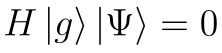
Find two instances of undetectable states:
In[]:=
FindInstanceWith{ψ=(a+b)@QuantumState[Flatten@Array[c,{$FockSize,$FockSize},{0,0}],{$FockSize,$FockSize}]},@ψ["Scalar"]==0,Flatten@Array[c,{$FockSize,$FockSize},{0,0}],2
†
ψ
Out[]=
c[0,0]--,c[0,1]-+,c[0,2]+,c[0,3]+,c[0,4]--,c[1,0]-,c[1,1]-+,c[1,2]--+,c[2,1]+,c[2,3]0,c[2,4]0,c[3,0]--,c[3,1]3+9,c[3,2]0,c[3,3]0,c[3,4]0,c[4,0]--,c[4,1]0,c[4,2]0,c[4,3]0,c[4,4]0,c[0,0]--,c[0,1]-5-,c[0,2]--,c[0,3]--,c[0,4]--,c[1,0]5+,c[1,1],c[1,2]++2,c[1,4]0,c[2,0]--,c[2,1]---2,c[2,3]0,c[2,4]0,c[3,0]+,c[3,1]+2,c[3,2]0,c[3,3]0,c[3,4]0,c[4,0]--,c[4,1]0,c[4,2]0,c[4,3]0,c[4,4]0
17
5
23
10
48
5
57
10
9
10
24
5
16
5
8
5
3
2
9
2
48
5
57
10
9
5
48
5
2
16
5
8
5
3
,c[1,3]3+9,c[1,4]0,c[2,0]9
10
24
5
16
5
8
5
3
,c[2,2](-3-9)3
2
16
5
8
5
3
2
9
2
29
10
2
23
10
5
2
19
10
3
2
14
5
21
10
23
10
5+
19
5
2
3
2
14
5
3
,c[1,3]21
5
5
2
19
10
3
2
14
5
3
,c[2,2]-21
5
3
2
3
2
14
5
21
5
21
10
Two mode case: Defining Bright and Dark States of Light
Two mode case: Defining Bright and Dark States of Light
The main purpose of this section is to introduce two types of states: states that are undetectable (dark states) and states that are detectable (bright states).
Consider a larger truncation of Fock space:
In[]:=
SetFockSpaceSize[10];
Symmetric and antisymmetric collective operators:
In[]:=
c:=(a+b)+b)
θ
2
;d:=(-a-θ
2
;The following commutators hold:
In[]:=
Commutator[a,b]
Out[]=
0
In[]:=
Commutator[c,d]
Out[]=
0
The transformation of operators must conserve number of photons, so for the two modes 〈 a+b = 〈 c+d
†
a
†
b
†
c
†
d
In[]:=
randomState=QuantumState["RandomPure",{$FockSize,$FockSize}]
Out[]=
QuantumState


In[]:=
Chop@@a+@b@randomState["Scalar"]
†
randomState
†
a
†
b
Out[]=
8.6897
In[]:=
ChopSimplify@@c+@d@randomState["Scalar"]
†
randomState
†
c
†
d
Out[]=
8.6897
Collective states defined for , fixing some number of maximum photons :
0<=n<=N
N
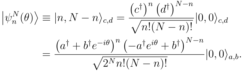
(
4
)Code representation of :
In[]:=
ClearAll[ψNn]ψNn[N_,n_]/;0<=n<=N<$FockSize:=Blockstate=FockState[{0,0}]["StateVector"],dMat=["Matrix"],cMat=["Matrix"],If[N-n>0,state=MatrixPower[dMat,N-n,state]];If[n>0,state=MatrixPower[cMat,n,state]];QuantumStateSimplify[Normal@state,θ∈Reals]
†
d
†
c
n!(N-n)!
,{$FockSize,$FockSize},"Parameters"->θNote can be max (that is the truncation constraint).
N
$FockSpace-1
One can show that:
(
5
)Check above equation for some cases:
In[]:=
With{Np=$FockSize-1},TableSum√(k!(Np-k)!)(n!(Np-n)!)SumBinomial[n,j]Binomial[Np-n,k-j],{j,Max[0,k-(Np-n)],Min[n,k]}QuantumTensorProduct[FockState[k],FockState[Np-k]],{k,0,Np}["StateVector"]==Simplify[Normal[ψNn[Np,n]["StateVector"]]],{n,0,Np}
θ(k-n)
Np
2
k-j
(-1)
Out[]=
{True,True,True,True,True,True,True,True,True,True}
We will use the new definition of since in the previous one, the matrix exponentials are computationally costly.
In[]:=
ClearAll[ψNn]ψNn[_,n_]/;0<=n<=<$FockSize:=QuantumStateSum,{j,Max[0,k-(-n)],Min[n,k]}QuantumTensorProduct[FockState[k],FockState[-k]],{k,0,},"Parameters"->θ
θ(k-n)
k!(-k)!
n!(-n)!
SumBinomial[n,j]Binomial[-n,k-j]
2
k-j
(-1)
For a given total number of photons N, the states form a complete basis ():
N
ψ
n
In[]:=
TableTableSimplify@ψNn[Np,j]["Scalar"],{i,0,Np},{j,0,Np}==IdentityMatrix[Np+1],{Np,$FockSize-1}
†
ψNn[Np,i]
Out[]=
{True,True,True,True,True,True,True,True,True}
Show
Mean value of number operator for mode-a
Checking the amplitudes of the analytical expression hold (“AmplitudeList” returns non zero amplitudes):
Checking the analytic expression for amplitudes:
Hamiltonian for two modes involving the interaction part:
Explaining double-slit: Interference from coherence, not from a “wavefront”
Explaining double-slit: Interference from coherence, not from a “wavefront”
The central, and rather provocative, claim of the paper is that “the interference of a single photon is not a signature of the wave character of the radiation.” What they show, in essence, is that everything you normally think of as “wave behavior” in the double-slit (the fringes!) can be derived purely from the quantum correlation functions of the light field and the process of photon detection, without ever having to ascribe a classical, propagating wave to the photon itself.
Double slit diagram:
Single photon case:
Single photon case:
For the simple case of one-photon, one gets:
The positive-frequency field operator at the detector screen is a superposition of the two “slit modes”:
Therefore, one gets:
But one can also rewrite Eq.12 as follows
Confirm Eq.16 (now including normalization):
Including a global phase can be expressed in this manner, if we call δ = θ - ϕ it possible to get only dark or bright state or a superposition depending on δ:
Note that the mean-value of number operators for mode-a and mode-b are non-zero, so it implies that photons are there, but not detectable.
Coherent state case:
Coherent state case:
Two mode not normalized coherent state with arbitrary amplitudes:
Decomposing the state using a change of basis to collective states, we get only bright states:
Since we used not normalized coherent states, we are not considering the normalization constant so we compare amplitudes up to that constant:
Symbolically we check the equation, but the truncation introduces residual errors in the “edges” (representing all the amplitudes as a matrix):
And two coherent states with opposite phases decompose only in the PDS subspace
Decomposing in the collective states basis, we get only dark states:
Checking amplitudes values:
This can be interpreted as destructive interference for two fields with same amplitude but opposite phases
Naturally this superposition of dark states has to be undetectable:
Verifying this fact:
In the context of the two slit experiment used with coherent states, can be described by a two mode coherent state with the same |α| but a relative phase dependent on the geometry of the slits and detection point (see diagram in single photon case)
In general in the collective basis this state has all components:
Detectable destructive interference
Detectable destructive interference
Not every state destructive interference field is undetectable, for example the state
Zero mean electric field (just using the part related to annihilation and creation operators):
We can see the decomposition of this state in that basis, has bright state component which is clearly detectable:
Other collective states: difference between classical and quantum
Other collective states: difference between classical and quantum
In general other collective states that are not MSS or PDS, cannot be related to classical fields or coherent states
We will evolve it in a MZI(Mach-Zehnder interferometer):
Symmetric beam splitter unitary:
Phase operator unitary:
MZI operator:
CITE THIS NOTEBOOK
CITE THIS NOTEBOOK
Bright and dark states of light: reinterpreting interference
by Bruno Tenorio
Wolfram Community, STAFF PICKS, May 16, 2025
https://community.wolfram.com/groups/-/m/t/3461741
by Bruno Tenorio
Wolfram Community, STAFF PICKS, May 16, 2025
https://community.wolfram.com/groups/-/m/t/3461741