Extending Stephen Wolfram's work on evolutionary selection of one-dimensional cellular automaton rules, this project seeks to explore mutations to rules for two-dimensional cellular automata. The project implements functionality to mutate CA rules one bit at a time, to find the shortest path between two rules when the full rule space is known, and an artificial survival of the fittest selection module to evolve 2D CAs according to a specified fitness function. We hope our project encourages the reader to investigate pattern mutations in cellular automata.
The One-Dimensional Case
The One-Dimensional Case
Setting the tone.
Setting the tone.
We begin by motivating this investigation with 1D CAs and learning how to “mutate” the rules at each possible step.
We begin by motivating this investigation with 1D CAs and learning how to “mutate” the rules at each possible step.
Below is a function that takes in a list of rules as an input and applies those rules in sequence to the initial conditions. For further context, we count the number of possible 1D CA rules, then, we move on to the 2D case.
In[]:=
ClearAll[caRuleCount1D]caRuleCount1D[colors_,range_]:=colors^colors^(2range+1);
In[]:=
ClearAll[caRuleCount2D]caRuleCount2D[colors_,range_]:=colors^colors^(2range+1)^2;
Show elementary CA rule mutations:
In[]:=
ClearAll[showRuleMutations]showRuleMutations[ruleNumber_]:=With[{rule=IntegerDigits[ruleNumber,2,8]}, (*Starting from a CA rule, list all possible mutations from that rule, and represent them in their base 10 form:*) FromDigits[#,2]&/@(ReplaceAt[rule,bit_:>If[bit==1,0,1],#]&/@Range[8])] (*Example:*)showRuleMutations[30]
Choose a random elementary CA 1 bit mutation:
In[]:=
ClearAll[randomRuleMutation1D]randomRuleMutation1D[ruleNumber_Integer]:=RandomChoice[showRuleMutations[ruleNumber]]
Here we define a function to show possible mutations of 1 bit from a starting rule:
In[]:=
ClearAll[showRuleMutationRules]showRuleMutationRules[ruleNumber_]:=With[{rule=IntegerDigits[ruleNumber,2,8]}, (*Starting from a CA rule, list all possible mutations from that rule, and represent them as rule->newRule:*) Map[rule#&,(ReplaceAt[rule,bit_:>If[bit==1,0,1],#]&/@Range[8])]]
To build intuition and set a strong conceptual foundation, we first consider one-dimensional cellular automata. We then work our way up to more complex cases of cellular automaton evolution.
In[]:=
ClearAll[applyMultipleCARules]applyMultipleCARules[init_List, listOfRules_List]:= FoldList[CellularAutomaton[#2,#1]&,init,listOfRules]
Furthermore, here are two visual examples, that we hope will provide the reader with a more cohesive visual picture underlying the code, and help aid with understanding how iterative mutations work on the starting rules.
Example 1:
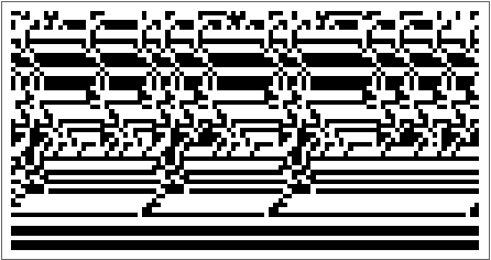
Start with a random initial condition, and and apply a sequence of random rules:
In[]:=
SeedRandom[1];ArrayPlot[applyMultipleCARules[RandomInteger[{0,1},100],RandomInteger[{0,255},50]],ColorRules{0White,1Black}]
Out[]=
Out[]=
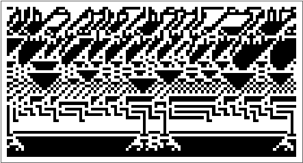
Example 2:
Start with a random initial condition, and apply a sequence of rules derived from successive mutations of a single rule:
In[]:=
SeedRandom[1];ArrayPlot[applyMultipleCARules[RandomInteger[{0,1},100],NestList[randomRuleMutation1D,30,50]],ColorRules{0White,1Black}]
Out[]=
Building Intuition - Paths and Distances Between Elementary CA Rules:
Building Intuition - Paths and Distances Between Elementary CA Rules:
In this section we aim to build intuition about the space of elementary cellular automaton rules and their mutations from one another.
We declare a variable elementaryCARules which stores the binary representation of every elementary CA rule.
In[]:=
elementaryCARules = Tuples[{0,1},{8}];
And here we define a list of possible mutations from every elementary CA rule:
In[]:=
ruleMutationLists=showRuleMutationRules/@Range[0,255];
A graph representing possible mutations from every elementary CA rule to every other:
In[]:=
ruleMutationsGraph=Graph3D[DeleteDuplicates[Sort/@Flatten[ruleMutationLists]]]
Out[]=

Here is some extra information about the graph itself:
In[]:=
{VertexCount[ruleMutationsGraph],EdgeCount[ruleMutationsGraph]}
Out[]=
{256,1024}
This is some code to find the shortest path through the graph between two rules:
In[]:=
Module[{start,end,shortestPath},{start,end}=RandomSample[elementaryCARules,2];shortestPath=FindShortestPath[ruleMutationsGraph,#1,#2]&@@{start,end};{HighlightGraph[ruleMutationsGraph,PathGraph[shortestPath],PlotLabel->("Path from "<>ToString[FromDigits[start,2]]<>" to "<>ToString[FromDigits[end,2]])],"PathLength"->Length[shortestPath]}]
Out[]=
 ,PathLength4
A CA fitness test for the evolving two-dimensional cellular automata.
A CA fitness test for the evolving two-dimensional cellular automata.
In this section, we search for two-dimensional CA rules that minimise distance to a goal by randomly mutating these rules and accepting the mutated rule if it exhibits better fitness. The testFitness function looks for CAs with slower rates of growth.
List rule mutations:
In[]:=
ClearAll[ruleMutations]ruleMutations[rule_Integer]:=BitXor[2^(Range[0,2^9-1]),rule]
Mutate a rule:
In[]:=
ClearAll[mutateRule]mutateRule[rule_Integer]:=BitXor[2^(RandomInteger[{0,2^9-1}]),rule]mutateRule[rule_List]:=Prepend[Rest[rule],mutateRule[First[rule]]](*mutateRule[0];mutateRule[{0,2,{1,1}}];*)
We want the fitness value with this configuration to be lower. In this example, higher fitness corresponds to lower fitness function values, as the fitness function returns the rate of growth over a defined interval of the dimensions of the minimal bounding 2D array that contains the last step of a candidate 2D CA.
Of course, if we were to change the fitness function, this might affect the kinds of comparisons that need to be made in the evolutionary process to pick rules with increasing fitness.
Another key aspect we look at is rules that quickly die out or keep going indefinitely. For our purposes, we want to get rid of these, since they either run for too long to be useful, or die out in the first steps.
In[]:=
ClearAll[testFitness]testFitness[rule_Integer,n_Integer:100,init_List:{{1}}]:=Module[{out,dims}, out=(*EchoFunction[ListAnimate[ArrayPlot/@#]&]@*)CellularAutomaton[{rule,2,{1,1}},{init,0},{n}]; dims=Dimensions[Last[out]]; Which[ (*If the result is an empty list, reject the rule:*) TrueQ[Length[out]==0],∞, (*If the last CA state is found at any previous step, reject the rule:*) MemberQ[Most[out],Last[out]],∞, (*If the result dimensions are {1,_}||{_,1}, reject the rule:*) MemberQ[dims,1],∞, (*Otherwise, return the dimensions of the final array divided by the number of computed steps:*) True,Times@@dims ]] testFitness[rule_List,n_Integer:100,init_List:{{1}}]:=testFitness[First[rule],n,init];
Here, we have commented out some draft code in order to assess the complexity of the last state of the CA using Shannon entropy.
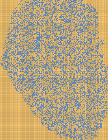
We initialize a way to generate visual examples of 2D cellular automata.
In[]:=
depthSetting=5000;ProgressIndicator[Dynamic[i],{0,depthSetting}]
Out[]=
You can change the depth, cut, and initRule parameters to get different outputs in the CA generator!
In[]:=
i=0;evolved=Module[{depth=depthSetting,cut=12,initRule=31(*RandomInteger[{0,Integer[]}]*)(*0*),initCond={{1}},ru,fitness,data},SeedRandom[1];evo=NestList[CompoundExpression[(*Incrementthecounter:*)i++,(*Mutatetheruleinputasthefirstargument:*)ru=mutateRule[First[#]],(*TeststhefitnessoftheCAuptothenumberofstepsdefinedbycut:*)fitness=testFitness[ru,cut,initCond],If[fitness<=Last[#],{ru,fitness},#]]&,{{initRule,2,{1,1}},∞},depth];evo=Rest[First/@SplitBy[evo,Last]];Map[CompoundExpression[data=CellularAutomaton[First[#],{initCond,0},{{{cut}}}],ArrayPlot[data,ColorRules->{0White,1Black},ImageSize->{Automatic,26Sqrt[Length[data]+1]},Mesh->True,MeshStyle->Opacity[.1]]]&,evo]];%//If[Length[#]>0,ListAnimate[#],#]&
Out[]=

In[]:=
caSims=(ArrayPlot[#,ColorRules{0White,1Black}]&/@CellularAutomaton[{#,2,{1,1}},{{{1}},0},15]&/@evo[[All,1,1]]);S(*ListAnimate/@%*)Export[FileNameJoin[{NotebookDirectory[],#2<>".gif"}],#1,"GIF"]&@@@Thread[{caSims,ToString/@evo[[All,1,1]]}]
In[]:=
Thread[{caSims,ToString/@evo[[All,1,1]]}]//Dimensions
We also leave the option for the reader to export the animation as a GIF:
In[]:=
Export[FileNameJoin[{NotebookDirectory[],"evolution.gif"}],evolved,"GIF"]
In[]:=
"/home/tor666/Desktop/CommunityPostUpdates/evolution.gif"//SystemOpen
The complex search for fitness.
The complex search for fitness.
There are a few reasons it’s hard to evolve 2D CAs for a particular fitness measure.
First, it’s difficult to define a fitness measure that results in the selection of CAs according to a meaningful criteria, as most 2D CAs will grow without bounds with stable boundary conditions, and a high degree of randomness. Then, it’s also difficult because the rule space is huge and there’s a good chance that we are spending the majority of the mutation time testing rules that are no good.
First, it’s difficult to define a fitness measure that results in the selection of CAs according to a meaningful criteria, as most 2D CAs will grow without bounds with stable boundary conditions, and a high degree of randomness. Then, it’s also difficult because the rule space is huge and there’s a good chance that we are spending the majority of the mutation time testing rules that are no good.
Concluding Remarks
Concluding Remarks
In conclusion, the key finding of the project has been the difficulty of scaling mutating cellular automata from the one-dimensional to the two-dimensional case. It’s unclear what heuristics may help to design better fitness measures. In this exploration, we defined fitness as the lowest array size after n steps. While there are 256 possible cases of one-dimensional CA rules, the two-dimensional cases grow significantly in complexity, which leaves us with questions about pattern mutations as we further increase the dimensionality of the CAs.
Acknowledgments
Acknowledgments
I’d like to acknowledge my mentors Phileas Dazeley-Gaist, and Christian Pasquel, who have been encouraging, educational, insightful, and inspiring from beginning to end. A special thanks to TA’s Lina M. Ruiz G. and Sebastian Rodriguez, who helped me with crucial questions and provided extra support. I would also like to mention Hatem Elshatlawy and Xerxes Arsiwalla for inspiring extra ideas throughout the project. Thanks to Stephen Wolfram for suggesting the project direction.
References
References
1
.S. Wolfram (2024), “Why Does Biological Evolution Work? A Minimal Model for Biological Evolution and Other Adaptive Processes” https://writings.stephenwolfram.com/2024/05/why-does-biological-evolution-work-a-minimal-model-for-biological-evolution-and-other-adaptive-processes/
2
.J. von Neumann (1966), “Theory of Self-Reproducing Automata,” University of Illinois Press. https://fab.cba.mit.edu/classes/865.18/replication/Burks.pdf
Cite This Notebook
Cite This Notebook