The idea of the simulation is that Maksimovich creates a reference space for many identical double pendulum systems albeit with different initial condition.
Use the initial condition works as index for each system.Then you release all pendulums at the same time and record the new [t] and [t] for each system at time . Also each pair of angles is encoded by a specific color, as shown below.
{[0],[0]}
θ
1
θ
2
θ
1
θ
2
t
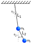
For example, a double pendulum starts with horizontal configure, = , is encoded green. After some time it moves to , then the point will change to like dark purple. So the animation is about such color permutation for all points on the plane and it evolves with time.
{[0],[0]}
θ
1
θ
2
{π/2,π/2}
{-π/2,π/3}
{π/2,π/2}
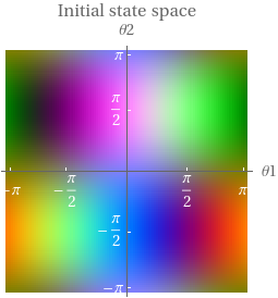
Create the reference color space
Create the reference color space
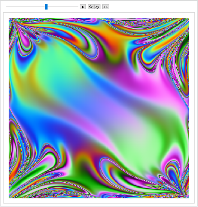
Color encoding of the initial state space:
In[]:=
initialAngleSet=Table[{θ1,θ2},{θ1,-π+0.01,π,0.02},{θ2,-π+0.01,π,0.02}];
In[]:=
getColor[θ1_,θ2_]:={Floor[127+127*Cos[θ2]*Sin[θ1]],Floor[127+127*Sin[θ2]*Sin[θ1]],Floor[127+127*Cos[θ2]]}/255.
I use the same normalized color scheme from the original source code by Maksimovich. The Graphics function in comment is the actual command to generate the color map below. I put the result in the numerical array object to cache the data so it won’t be affected if I upgrade the resolution for the .
initialAngleSet
In[]:=
(*Graphics[Raster[Downsample[Apply[getColor,initialAngleSet,{2}],{3,3,1}]]]*)GraphicsRasterNumericArray,,AxesLabel{θ1,θ2}
Out[]=
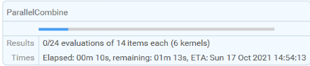
Solving 100000+ ODE’s in parallel
Solving 100000+ ODE’s in parallel
This is the differential equation that describes the dynamics of the double pendulum from StackExchange (θ is same as ϕ in the code):
In[]:=
sol=ParametricNDSolveValue[{2*phi1''[t]+phi2''[t]*Cos[phi1[t]-phi2[t]]+phi2'[t]^(2)*Sin[phi1[t]-phi2[t]]+2*9.81*Sin[phi1[t]]==0,phi2''[t]+phi1''[t]*Cos[phi1[t]-phi2[t]]-phi1'[t]^(2)*Sin[phi1[t]-phi2[t]]+9.81*Sin[phi2[t]]==0,phi1[0]==θ1Init,phi2[0]==θ2Init,phi1'[0]==0,phi2'[0]==0},{phi1,phi2},{t,0,5},{θ1Init,θ2Init}];
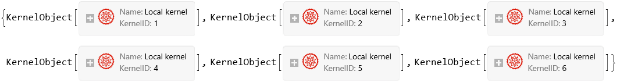
Use parallel kernels to accelerate the process:
In[]:=
LaunchKernels[]
Out[]=
Physically, the following is equal to release all double pendulums at the same time. This is the only line you need to trigger the solver to convert the into numerical interpolation for each initial condition. On my six core machine the computation gets around 4.85 times acceleration to actually solve each ODE system with different initial condition. It takes around 50 seconds to finish solving 10000+ ODE’s, each simulates a double pendulum system for 5 seconds.
ParametricFunciton
interpolations=Parallelize[Apply[sol[#1,#2]&,initialAngleSet,{2}]];
It is nice to see a progress bar on later versions to handle long computation.
The last step is to render in parallel for the whole process for each initial condition. This step takes slightly more than 1 minute if I choose use to push all interpolation function to subkernels first. The parallel computation takes about 45 seconds (with 5.5 speed up) and rest are for master kernel combining the results from the subkernels. is the key to create a very short code to extract numerical value for each system at a given time point:
DistributeDefinitions
MapThread
In[]:=
frames=ParallelTable[Image[Apply[getColor,MapThread[#1@#2&,{interpolations,ConstantArray[t,Dimensions[interpolations]]},3],{2}],ImageSize500],{t,0,5,0.1}];
Create animation:
In[]:=
ListAnimate[frames]
Out[]=
Profile for each system with distinct initial condition
Profile for each system with distinct initial condition
These are the lattice point for . Each point is an initial condition:
{-π,π}x{-π,π}
In[]:=
Dimensions[initialAngleSet]
Out[]=
{314,314,2}
Each point undergoes continuous color change (except ) associated with the phase diagram that describe the actual motion of the pendulum system in terms of angle. Besides the global pattern, we can profile each point by coloring its curve according to the reference color space:
{0,0}
◼
Some point close to {0,0}, which has mild swing and stable.
In[]:=
DirectionParametricPlot[Through[interpolations[[100,70]][p]],{p,0,5},ColorFunction->(RGBColor@@getColor[#1,#2]&),ColorFunctionScaling->False,"ArrowSize"->1.3,"ArrowNumber"->8]
Out[]=
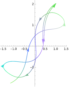
◼
Some point close to {π/2,π}. Now our pendulum system is L shape. The phase diagram is more divergent than the above.
In[]:=
314*0.75//Floor
Out[]=
235
In[]:=
plt=DirectionParametricPlot[Through[interpolations[[235,314]][p]]//Evaluate,{p,0,5},ColorFunction->(RGBColor@@getColor[#1,#2]&),ColorFunctionScaling->False,"ArrowSize"->1.3,"ArrowNumber"->20]
Out[]=
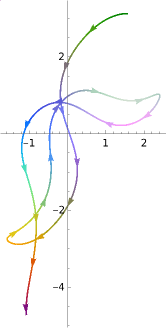
Notice how the color on each curve matches the color scheme in each quadrant of the reference color space.
Close kernels to clear cache on sub kernels:
In[]:=
CloseKernels[]
Out[]=
Summary
Summary
◼
Use Raster function to create color encoding for a 2D point
◼
ParametricNDSolve handles same dynamic system with different initial condition
◼
MapThread[#1@#2&.,...]
◼
CPU: Intel Xeon W-10855M @ 2.8GHZ to 5.1 GHZ + 72 GB RAM
Utility function
Utility function
Here is a modified version of the WFR function. It gives an improved version of ColorFunction support and equal-distance between points along any parameterized curve, which is very suitable for this application.
DirectionParametricPlot
Definition of Modified DirectionParametricPlot
Definition of Modified DirectionParametricPlot
Equal space along a parameterized curve
Equal space along a parameterized curve