GEO Projections are awesome, we can see maps of our orange shaped world in different perspectives.
First checking some definitions about GEO technology with GPT-4 LLM:
Define GEO projection in just one paragraph
A GEO projection, or geographic projection, is a method used in cartography to represent the curved surface of the Earth on a flat map. This transformation involves mathematical algorithms that convert the three-dimensional coordinates of the Earth's surface into two-dimensional coordinates, allowing for the visualization of geographical features. Various types of GEO projections exist, each with specific properties and uses, such as preserving area, shape, distance, or direction. Common projections include the Mercator, which preserves angles, and the Robinson, which provides a more visually appealing representation of the entire world. These projections are essential for creating accurate and useful maps for navigation, education, and geographic analysis.
Define GEO processing in just one paragraph
GEO processing, or geospatial processing, refers to the manipulation and analysis of geographic data through computational techniques. This process involves transforming raw geospatial data into useful information by applying various algorithms and operations, such as data cleaning, transformation, analysis, and visualization. GEO processing can include tasks like spatial analysis, terrain modeling, map overlay, and network analysis, which are essential for understanding spatial relationships and patterns across different geographic regions. It is widely used in fields such as urban planning, environmental monitoring, transportation, and disaster management, enabling decision-makers to gain insights and make informed decisions based on geographic information.
In the context of Data Science define geographic analysis in one paragraph
In the context of data science, geographic analysis involves the exploration and examination of spatial data to uncover patterns, relationships, and insights that are geographically or spatially significant. This type of analysis leverages geospatial data, which includes information about the location and characteristics of features on the Earth's surface, to address complex questions and problems. Techniques used in geographic analysis include spatial statistics, geostatistics, geographic information systems (GIS), and spatial data visualization. By integrating geographic analysis into data science workflows, practitioners can identify spatial trends, optimize resource allocation, assess environmental impacts, and enhance decision-making processes across diverse fields such as urban planning, public health, transportation, and market analysis.
For convenience Wolfram Language set by itself the appropriate GEO projection according the ZOOM for GeoGraphics:
In[]:=
?GeoGraphics
Out[]=
In[]:=
GeoGraphics[GeoMarker[Here],GeoRangeQuantity[1,"Miles"]]
Out[]=
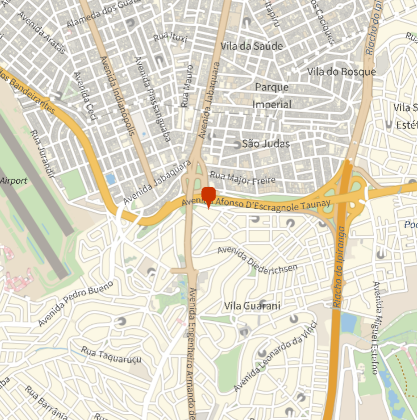
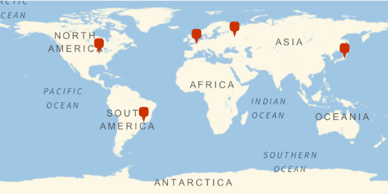
We can see the world, and mark some interesting places, getting curated data from Wolfram|Alpha, using Entity:
In[]:=
GeoGraphics[GeoMarker/@{Here,(=[Urbana]),(=[Paris]),(=[Moscow]),(=[Tokio])},GeoRange"World"]
Out[]=
Wolfram Language has more than 500 different projections:
In[]:=
Length[GeoProjectionData[]]
Out[]=
532
We can list the projections available:
In[]:=
GeoProjectionData[]
Out[]=
{Airy,Aitoff,Albers,AmericanPolyconic,ApianI,ApianII,ArdenClose,Armadillo,AugustEpicycloidal,AzimuthalEquidistant,BaconGlobular,Balthasart,BehrmannEqualArea,BipolarObliqueConicConformal,BoggsEumorphic,Bonne,Bottomley,BraunConicStereographic,BraunCylindrical,BraunII,BSAMCylindrical,Cassini,Collignon,ConicEquidistant,ConicPerspective,ConicSatelliteTracking,CraigRetroazimuthal,Craster,CrasterCylindricalEqualArea,CylindricalEqualArea,CylindricalEquidistant,CylindricalPerspective,CylindricalSatelliteTracking,DenoyerSemielliptical,EckertGreifendorff,EckertI,EckertII,EckertIII,EckertIV,EckertV,EckertVI,EqualEarth,EquatorialStereographic,Equirectangular,Euler,FoucautEqualArea,FoucautStereographic,FournierGlobularI,FournierII,GallIsographic,GallStereographic,GinzburgI,GinzburgII,GinzburgIV,GinzburgIX,GinzburgPseudoCylindrical,GinzburgV,GinzburgVI,Gnomonic,GoodeHomolosine,GottElliptical,GottMugnoloElliptical,Hammer,Hatano,HerschelConicConformal,HoboDyer,Hyperelliptical,KarchenkoShabanova,KavrayskiyV,KavrayskiyVII,Lagrange,LambertAzimuthal,LambertConicConformal,LambertConicConformalBelgium,LambertConicConformalNGS,LambertConicEqualArea,LambertConicNearConformal,LambertCylindrical,Larrivee,Littrow,Loximuthal,Maurer,McBrydeThomasFlatPolarParabolic,McBrydeThomasFlatPolarQuartic,McBrydeThomasFlatPolarSinusoidal,McBrydeThomasI,McBrydeThomasII,Mercator,MillerCylindrical,MillerCylindricalII,MillerPerspective,Mollweide,MurdochI,MurdochII,MurdochIII,NaturalEarth,Nell,NellHammer,ObliqueMercator,ObliqueMercatorNGS,OrteliusOval,Orthographic,PavlovCylindrical,PeirceQuincuncial,PutninsP1,PutninsP1Prime,PutninsP2,PutninsP3,PutninsP3Prime,PutninsP4Prime,PutninsP5,PutninsP5Prime,PutninsP6,PutninsP6Prime,QuarticAuthalic,RectangularPolyconic,Robinson,Shield,SinuMollweide,Sinusoidal,SnyderMinimumError,SpaceObliqueMercator,SPCS27AK01,SPCS27AK02,SPCS27AK03,SPCS27AK04,SPCS27AK05,SPCS27AK06,SPCS27AK07,SPCS27AK08,SPCS27AK09,SPCS27AL01,SPCS27AL02,SPCS27AR01,SPCS27AR02,SPCS27AZ01,SPCS27AZ02,SPCS27AZ03,SPCS27CA01,SPCS27CA02,SPCS27CA03,SPCS27CA04,SPCS27CA05,SPCS27CA06,SPCS27CA07,SPCS27CO01,SPCS27CO02,SPCS27CO03,SPCS27CT00,SPCS27DE00,SPCS27FL01,SPCS27FL02,SPCS27FL03,SPCS27GA01,SPCS27GA02,SPCS27HI01,SPCS27HI02,SPCS27HI03,SPCS27HI04,SPCS27HI05,SPCS27IA01,SPCS27IA02,SPCS27ID01,SPCS27ID02,SPCS27ID03,SPCS27IL01,SPCS27IL02,SPCS27IN01,SPCS27IN02,SPCS27KS01,SPCS27KS02,SPCS27KY01,SPCS27KY02,SPCS27LA01,SPCS27LA02,SPCS27LA03,SPCS27MA01,SPCS27MA02,SPCS27MD00,SPCS27ME01,SPCS27ME02,SPCS27MI01,SPCS27MI02,SPCS27MI03,SPCS27MI11,SPCS27MI12,SPCS27MI13,SPCS27MN01,SPCS27MN02,SPCS27MN03,SPCS27MO01,SPCS27MO02,SPCS27MO03,SPCS27MS01,SPCS27MS02,SPCS27MT01,SPCS27MT02,SPCS27MT03,SPCS27NC00,SPCS27ND01,SPCS27ND02,SPCS27NE01,SPCS27NE02,SPCS27NH00,SPCS27NJ00,SPCS27NM01,SPCS27NM02,SPCS27NM03,SPCS27NV01,SPCS27NV02,SPCS27NV03,SPCS27NY01,SPCS27NY02,SPCS27NY03,SPCS27NY04,SPCS27OH01,SPCS27OH02,SPCS27OK01,SPCS27OK02,SPCS27OR01,SPCS27OR02,SPCS27PA01,SPCS27PA02,SPCS27PR01,SPCS27PR02,SPCS27RI00,SPCS27SC01,SPCS27SC02,SPCS27SD01,SPCS27SD02,SPCS27TN00,SPCS27TX01,SPCS27TX02,SPCS27TX03,SPCS27TX04,SPCS27TX05,SPCS27UT01,SPCS27UT02,SPCS27UT03,SPCS27VA01,SPCS27VA02,SPCS27VT00,SPCS27WA01,SPCS27WA02,SPCS27WI01,SPCS27WI02,SPCS27WI03,SPCS27WV01,SPCS27WV02,SPCS27WY01,SPCS27WY02,SPCS27WY03,SPCS27WY04,SPCS83AK01,SPCS83AK02,SPCS83AK03,SPCS83AK04,SPCS83AK05,SPCS83AK06,SPCS83AK07,SPCS83AK08,SPCS83AK09,SPCS83AK10,SPCS83AL01,SPCS83AL02,SPCS83AR01,SPCS83AR02,SPCS83AZ01,SPCS83AZ02,SPCS83AZ03,SPCS83CA01,SPCS83CA02,SPCS83CA03,SPCS83CA04,SPCS83CA05,SPCS83CA06,SPCS83CO01,SPCS83CO02,SPCS83CO03,SPCS83CT00,SPCS83DE00,SPCS83FL01,SPCS83FL02,SPCS83FL03,SPCS83GA01,SPCS83GA02,SPCS83HI01,SPCS83HI02,SPCS83HI03,SPCS83HI04,SPCS83HI05,SPCS83IA01,SPCS83IA02,SPCS83ID01,SPCS83ID02,SPCS83ID03,SPCS83IL01,SPCS83IL02,SPCS83IN01,SPCS83IN02,SPCS83KS01,SPCS83KS02,SPCS83KY01,SPCS83KY02,SPCS83LA01,SPCS83LA02,SPCS83LA03,SPCS83MA01,SPCS83MA02,SPCS83MD00,SPCS83ME01,SPCS83ME02,SPCS83MI11,SPCS83MI12,SPCS83MI13,SPCS83MN01,SPCS83MN02,SPCS83MN03,SPCS83MO01,SPCS83MO02,SPCS83MO03,SPCS83MS01,SPCS83MS02,SPCS83MT00,SPCS83NC00,SPCS83ND01,SPCS83ND02,SPCS83NE00,SPCS83NH00,SPCS83NJ00,SPCS83NM01,SPCS83NM02,SPCS83NM03,SPCS83NV01,SPCS83NV02,SPCS83NV03,SPCS83NY01,SPCS83NY02,SPCS83NY03,SPCS83NY04,SPCS83OH01,SPCS83OH02,SPCS83OK01,SPCS83OK02,SPCS83OR01,SPCS83OR02,SPCS83PA01,SPCS83PA02,SPCS83PR00,SPCS83RI00,SPCS83SC00,SPCS83SD01,SPCS83SD02,SPCS83TN00,SPCS83TX01,SPCS83TX02,SPCS83TX03,SPCS83TX04,SPCS83TX05,SPCS83UT01,SPCS83UT02,SPCS83UT03,SPCS83VA01,SPCS83VA02,SPCS83VT00,SPCS83WA01,SPCS83WA02,SPCS83WI01,SPCS83WI02,SPCS83WI03,SPCS83WV01,SPCS83WV02,SPCS83WY01,SPCS83WY02,SPCS83WY03,SPCS83WY04,Stereographic,TiltedPerspective,Times,TissotConicEqualArea,ToblerI,ToblerII,TransverseMercator,TrapezoidalMercator,TrystanEdwards,UPSNorth,UPSSouth,UrmayevCylindricalII,UrmayevCylindricalIII,UrmayevI,UrmayevPseudoCylindrical,UTMZone01,UTMZone01South,UTMZone02,UTMZone02South,UTMZone03,UTMZone03South,UTMZone04,UTMZone04South,UTMZone05,UTMZone05South,UTMZone06,UTMZone06South,UTMZone07,UTMZone07South,UTMZone08,UTMZone08South,UTMZone09,UTMZone09South,UTMZone10,UTMZone10South,UTMZone11,UTMZone11South,UTMZone12,UTMZone12South,UTMZone13,UTMZone13South,UTMZone14,UTMZone14South,UTMZone15,UTMZone15South,UTMZone16,UTMZone16South,UTMZone17,UTMZone17South,UTMZone18,UTMZone18South,UTMZone19,UTMZone19South,UTMZone20,UTMZone20South,UTMZone21,UTMZone21South,UTMZone22,UTMZone22South,UTMZone23,UTMZone23South,UTMZone24,UTMZone24South,UTMZone25,UTMZone25South,UTMZone26,UTMZone26South,UTMZone27,UTMZone27South,UTMZone28,UTMZone28South,UTMZone29,UTMZone29South,UTMZone30,UTMZone30South,UTMZone31,UTMZone31South,UTMZone32,UTMZone32South,UTMZone33,UTMZone33South,UTMZone34,UTMZone34South,UTMZone35,UTMZone35South,UTMZone36,UTMZone36South,UTMZone37,UTMZone37South,UTMZone38,UTMZone38South,UTMZone39,UTMZone39South,UTMZone40,UTMZone40South,UTMZone41,UTMZone41South,UTMZone42,UTMZone42South,UTMZone43,UTMZone43South,UTMZone44,UTMZone44South,UTMZone45,UTMZone45South,UTMZone46,UTMZone46South,UTMZone47,UTMZone47South,UTMZone48,UTMZone48South,UTMZone49,UTMZone49South,UTMZone50,UTMZone50South,UTMZone51,UTMZone51South,UTMZone52,UTMZone52South,UTMZone53,UTMZone53South,UTMZone54,UTMZone54South,UTMZone55,UTMZone55South,UTMZone56,UTMZone56South,UTMZone57,UTMZone57South,UTMZone58,UTMZone58South,UTMZone59,UTMZone59South,UTMZone60,UTMZone60South,VanDerGrinten,VanDerGrintenII,VanDerGrintenIII,VanDerGrintenIV,VerticalPerspective,WagnerI,WagnerII,WagnerIII,WagnerIV,WagnerIX,WagnerV,WagnerVI,WagnerVII,WagnerVIII,WerenskioldI,Werner,Wiechel,WinkelI,WinkelII,WinkelSnyder,WinkelTripel}
Lets see just the first 10 of them:
In[]:=
Take[GeoProjectionData[],10]
Out[]=
{Airy,Aitoff,Albers,AmericanPolyconic,ApianI,ApianII,ArdenClose,Armadillo,AugustEpicycloidal,AzimuthalEquidistant}
Here we use a Wolfram Research Inc Entity function to get the company head quarters GEO coordinates:
In[]:=
wr=["Coordinates"]
Out[]=
{40.0979,-88.2457}
For Apple head quarters GEO coordinates, we try in a different way, to use NominatinmData from OpenStreepMap:
In[]:=
ResourceFunction["NominatimData"]["Apple Inc"]
Out[]=
{place_id311960903,licenceData © OpenStreetMap contributors, ODbL 1.0. http://osm.org/copyright,osm_typeway,osm_id33463538,lat37.3326452,lon-122.02992302100607,categorylanduse,typecommercial,place_rank22,importance0.407764,addresstypecommercial,nameApple Campus,display_nameApple Campus, Cupertino, Santa Clara County, California, United States,boundingbox{37.3303077,37.3339670,-122.0320420,-122.0277960}}
In[]:=
apple=ToExpression[First[Normal[Values[Dataset[%][All,{"lat","lon"}]]]]]
Out[]=
{37.3326,-122.03}
Using curated data from Wolfram|Alpha, we have a list of lat and log from some interesting places:
In[]:=
places={Here,wr,apple,(=[Paris]),(=[Moscow]),(=[Tokio])}
Out[]=
GeoPosition[{-23.63,-46.64}],{40.0979,-88.2457},{37.3326,-122.03},,,
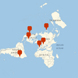
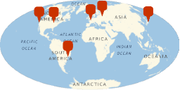
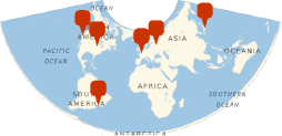
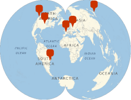
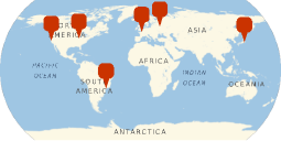
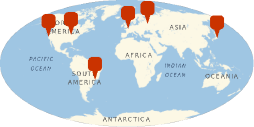
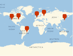
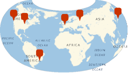
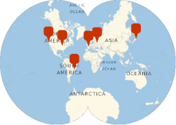
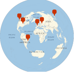
Visualizing those places coordinates with different GEO projections:
In[]:=
Grid@({#,GeoGraphics[GeoMarker/@places,GeoRange"World",GeoProjection->#]}&/@Take[GeoProjectionData[],10])
Out[]=
Airy | |
Aitoff | |
Albers | |
AmericanPolyconic | |
ApianI | |
ApianII | |
ArdenClose | |
Armadillo | |
AugustEpicycloidal | |
AzimuthalEquidistant |
To try each of the GEO projections available at Wolfram Language, we can use a GUI with Manipulate:
In[]:=
Manipulate[GeoGraphics[Insert[(GeoMarker/@places),Blue,2],GeoRange"World",GeoProjection->projection,ImageSize->400],{projection,GeoProjectionData[]},SaveDefinitions->True]
Out[]=
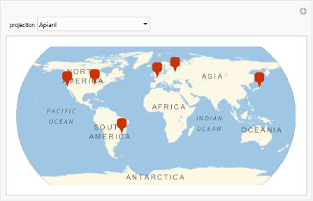
We are used to some of popular GEO projections, but some of than can see exotic!
GEO processing and cartographs personal are used to those unusual projections.
GEO processing and cartographs personal are used to those unusual projections.
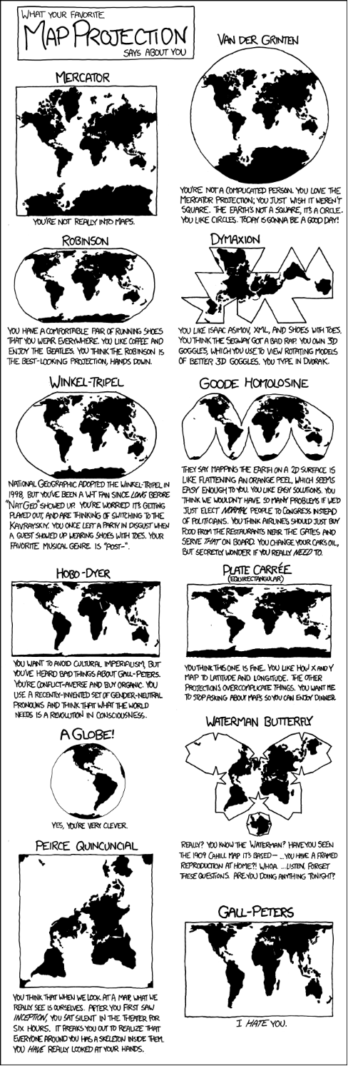
For a better understanding of GEO Projections, take a look at this funny infographic below, this is the inspiration for this post:
Source: https://xkcd.com/977/
CITE THIS NOTEBOOK
CITE THIS NOTEBOOK
Geo-projections as data: exploring visual and computational aspects of cartographic shapes
by Daniel Carvalho
Wolfram Community, STAFF PICKS, October 24, 2024
https://community.wolfram.com/groups/-/m/t/3305897
by Daniel Carvalho
Wolfram Community, STAFF PICKS, October 24, 2024
https://community.wolfram.com/groups/-/m/t/3305897