Air travel plays a crucial role in our everyday lives by connecting people and places, facilitating global trade, and enabling rapid travel. My research focuses on optimizing air travel efficiency by leveraging wind data to identify the most effective flight routes. I used WindVectorData and various Wolfram functions as resources for my work. These analyses provide insight into the impact of wind on air travel and how flight paths can be optimized to adapt to them. With this project, I hope to streamline the process of air travel. However, this project does not account for factors such as air resistance on the plane.
Introduction
Introduction
I still remember my first ride on a private plane. As we soared through the skies, I remembered the beautiful, orangish pink view of the sun setting under the clouds. But suddenly, all the clouds seemed to pass by and left only the busting cityscape beneath us. My neighbor, Eric, noticed my fascination and started to tell me about the role of weather on flight planning. Specifically, the wind remained a large topic of discussion. I’ve still remained fascinated by the complexity of it all, and it sparked a curiosity in me to learn more about the wind and its impact on air travel.
Wind patterns play a significant role in flight operations, often impacting flight schedules and causing delays. This inspired me to base my project off of the effect of wind. This project combines physics, map visualization, and real-time wind data to improve flight planning and reduce delays. I aim to improve flight times and streamline flight planning.
As a quick note, this simulation doesn’t account for several factors, such as air resistance and other atmospheric conditions. However, since these factors are uniformly ignored, everything remains relative, ensuring that the predicted flight times are accurate.
Visualizing Wind and Map Data
Visualizing Wind and Map Data
Depending on the direction and strength of the wind, planes can either be aided or hindered in their progress. By combining wind patterns with map data, pilots and air traffic controllers can create efficient routes.
WindVectorData provides current and historical wind vector data from standard weather stations worldwide. Wind vectors combine wind direction and speed into a two-component upwind velocity, with the components latitude and longitude. For example, this function can be used to check the current WindVector at the LAX airport.
In[]:=
WindVectorData
Out[]=
,
In addition to this, an airport’s wind data can be accessed from typing its name or its GeoPosition.
In[]:=
WindVectorData["KLAX"]WindVectorData[GeoPosition[{34,-118}]]
Out[]=
,
Out[]=
,
In a nutshell, WindVectorData is incredibly versatile, and is capable of being used for a wide range of applications and accepting various inputs. This functionality is particularly valuable when determining flight paths influenced by wind conditions.
Visualizing Direct Flight Paths
Visualizing Direct Flight Paths
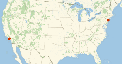
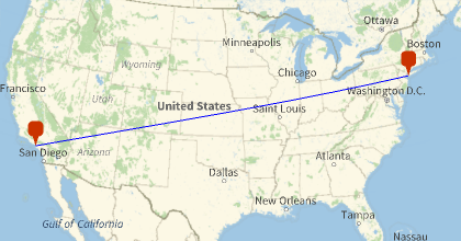
To gain a better picture of the difference between a direct and efficient flight path, I’ve generated an example of two points across the United States. To get a better representation of the wind data, I visualized these two points on a map using the GeoListPlot function, which will take two locations as inputs (in this case, the LAX and JFK airports) and generate a map displaying them.
In[]:=
GeoListPlot,
Out[]=
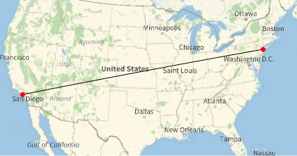
Next, GeoPath can be used to draw a path between the two points. This shows the direct flight path.
In[]:=
GeoGraphicsGeoPath,,Red,PointSize[Large],Point,Point
Out[]=
Random Point Generation
Random Point Generation
To generate the best flight paths, I needed a function that produces random points along the route, which diversifies the potential path options. This ensures that the generated paths are efficient and not randomly scattered, while also allowing for easy point generation.
randPointGenerator takes two locations as its input. It uses the coordinates as a boundary for the flight’s path. This was used to ensure that the plane didn’t go unnecessary paths.
Generates a random point using the starting and ending location that the user inputs.
In[]:=
randomPointGenerator[leave_,land_]:=Module[{xLeave,yLeave,xLand,yLand,rectangleList,orderList,latLongList,randChoc,randomMap,avgVector,avg1Vector,avg2Vector},xLeave=leave[[1,1]];xLeave=leave[[1,1]];yLeave=leave[[1,2]];xLand=land[[1,1]];xLeave=leave[[1,1]];yLand=land[[1,2]];If[xLeave>xLand&&yLeave>yLand,orderList=4,If[xLeave>xLand&&yLand>yLeave,orderList=3,If[xLand>xLeave&&yLand>yLeave,orderList=2,If[xLand>xLeave&&yLeave>yLand,orderList=1]]]];Switch[orderList,4,rectangleList=Table[{x,y},{x,xLand,4+xLeave},{y,yLand,yLeave}],3,rectangleList=Table[{x,y},{x,xLand,4+xLeave},{y,yLand,yLeave}],2,rectangleList=Table[{x,y},{x,xLeave,4+xLand},{y,yLeave,yLand}],1,rectangleList=Table[{x,y},{x,xLeave,4+xLand},{y,yLand,yLeave}]];latLongList=Partition[Flatten[rectangleList],2];randChoc=RandomChoice[latLongList];randChoc]
I tested the function by inputting a starting and ending location. The output shows a randomly generated point along the coordinate plane of these places.
Implements the function. Output shows a random point from the rectangle generated from JFK to LAX.
In[]:=
randomPointGenerator,
Out[]=
{34.9425,-85.4081}
Random Points on a Graph
Random Points on a Graph
This section generates a map that serves as a visual aid. With this, the user can see where the random points are being chosen.
First, I’ve individually defined JFK’s and LAX’s latitude and longitude. This is so they can be used to make a list of points.
In[]:=
latLAX=34;lonLAX=-118;latJFK=41;lonJFK=-74;
Next, I found the smaller and larger latitude and longitude. This is because the Range function takes points from smallest to largest as inputs.
In[]:=
latMin=Min[latLAX,latJFK];latMax=Max[latLAX,latJFK];lonMin=Min[lonLAX,lonJFK];lonMax=Max[lonLAX,lonJFK];
The resolution defines the frequency of the points. It can be thought of how “clear” the individual points are on the graph. The smaller the resolution, the denser the points.
In[]:=
resolution=0.75;
Then, I made a list of all the latitudes and longitudes, and combined them in a list using Table.
In[]:=
lats=Range[latMin,latMax+3,resolution];lons=Range[lonMin+3,lonMax,resolution];points=Flatten[Table[GeoPosition[{lat,lon}],{lat,lats},{lon,lons}],1];
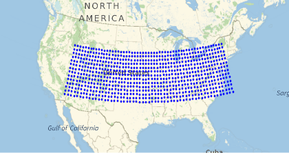
Finally, I’ll plot the points using the Point function. This shows the potential areas that the random points can be chosen from.
GeoGraphics{Blue,Point[points]},GeoRange->
Out[]=
Mathematical Functions
Mathematical Functions
Math, particularly physics, is essential for understanding the duration of the flight. This section of the project involves using common physics equations to make an estimate of the flight’s duration. I personally feel that I learnt the most in this section because of the need to understand the equations, implement them, and fix the computational errors that came with them.
Finding Average Vectors
Finding Average Vectors
Finding the average vector in a flight path is essential because it represents the overall direction and speed of the wind affecting the aircraft over the entire journey. This also corresponds to acceleration by indicating the net change in velocity due to wind forces over the flight path. To find the average vector over a curved path, one common function that I use is the BSplineFunction. This function helps generate smooth curves through the random points along the flight path.
Finds the average vector over a curved flight path.
In[]:=
avgVectorFunc[start_, randP_, land_] := Module[{latLongPairs, newXVals, newYVals, xVector, yVector, avgVector, planePath, windVectors}, planePath = BSplineFunction[{start[[1]], randP, land[[1]]}]; windVectors = Partition[ Flatten[QuantityMagnitude[ WindVectorData /@ Table[planePath[x], {x, 0, 1, 0.1}]] /. Missing["NotAvailable"] -> {0, 0}], 2]; newXVals = Total[windVectors[[All, 1]]]; newYVals = Total[windVectors[[All, 2]]]; xVector = newXVals/10; yVector = newYVals/10; avgVector = {xVector, yVector}]
To use this, the user can input an initial location, a randomly chosen point, and the desired destination.
Implements the function using LAX as the starting location, a random point, and JFK as the ending location.
In[]:=
avgVectorFunc,{36,-90},
Out[]=
{-1.44301,-0.624066}
The plane’s average vector provides information about the overall direction and magnitude of the plane over a specific period or distance. It helps to predict the net effect on an aircraft’s trajectory and speed. The plane’s speed is assumed to be 500 miles/hour.
Finds the average vector of the plane.
In[]:=
planeVectorSlope[start_,end_]:=N[500*Normalize[{end[[1,1]]-start[[1,1]],end[[1,2]]-start[[1,2]]}]]
This below calculation uses a method based on the Pythagorean theorem to compute the magnitude of a vector (the vector’s “strength”).
Calculates the magnitude of the vector with two user-inputted locations.
In[]:=
magnitude[{x_,y_}]:=Ifx<0||y<0,-+,+
2
x
2
y
2
x
2
y
Using the plane’s and average wind vector, this function determines the magnitude of the wind component parallel to the plane’s direction. I only considered the wind vector parallel to the plane to simplify calculations under varying wind conditions.
Determines the magnitude of the parallel wind component to the plane.
In[]:=
anglePlaneVector[u_List,v_List]:=Module{projection},projection=u;N[magnitude[projection]]
u.v
u.u
This following function finds the magnitude of the acceleration of the wind. This is essential for finding the flight duration, as it models the effect of the wind over the entire journey.
Finds the strength of the wind’s acceleration.
In[]:=
applyPlaneRand[start_,randP_,end_]:=anglePlaneVector[planeVectorSlope[start,end],avgVectorFunc[start,randP,end]]
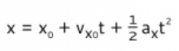
The approximate time a flight will take can be calculated using a re-arranged form of the position formula in physics. This is later used when finding the best flight path.
This is the original equation:Once again, I’ve assumed 500 mph as the plane speed.
Uses a re-arranged version of the position function to calculate the rough time a flight will take.
In[]:=
roughTime[start_,randP_,end_]:=(-500+Sqrt[500^2-2*applyPlaneRand[start,randP,end]*(-QuantityMagnitude[GeoDistance[start,end]])])/(applyPlaneRand[start,randP,end])
The user can test this function by inputting a starting location, a random point, and a destination. The output shows that the flight will take around 5 hours, or around 300 minutes.
Implements the function with a starting location, a random point, and an ending location. The output shows the computed time.
In[]:=
roughTime,{36,-90},
Out[]=
5.05032
A quick note, the actual flight time from LAX to JFK is 6.5 hours. As mentioned before, however, all values are relative. In theory, the flight should take 2474.89 (the distance in miles)/500 (speed in miles/hour), which is equal to 4.9 hours.
Finding the Best Path
Finding the Best Path
Many travelers have a familiar experience - waiting on a flight, feeling restless, and checking the flight’s progress only to be surprised by a curved path. But why do planes take these routes? One reason is the wind. By using wind patterns to their advantage, pilots can reduce fuel consumption, travel time, and emissions.
pathPlotter is used to find a path and it’s time. This uses the randomPointGenerator and calculates the time with roughTime. This is important for finding and plotting the best path later.
Returns the time it takes for a randomly generated path and a spline function.
In[]:=
pathPlotter[leave_,land_]:=Module[{totalTime,randPoint,locations,timeList},randPoint=randomPointGenerator[leave,land];totalTime=roughTime[leave,randPoint,land];locations=BSplineFunction[{leave[[1]],randPoint,land[[1]]}];{totalTime,locations}]
Running this (with two locations as the input) shows a random path and the time it will take for the plane to travel on this path.
In[]:=
pathPlotter,
5.0135,BSplineFunction
Finally, I created a function called findBestPath that uses PathPlotter to generate 10 distinct paths and then maps the one with the best time.
Generates random paths, finds the best one, and maps that one onto a map.
In[]:=
findBestPath[leave_,land_]:=Module[{allPath,times,bestTime,bestIndex,bestPath,randomMap},allPath=Table[pathPlotter[leave,land],{10}];times=allPath[[All,1]];bestTime=Min[times];bestIndex=FirstPosition[times,bestTime][[1]];bestPath=allPath[[bestIndex]][[2]];randomMap=With[{locations=bestPath},GeoGraphics[{{Blue,GeoPath[Table[locations[x],{x,0,1,0.1}]],{Red,GeoMarker[leave]},{Red,GeoMarker[land]}},GeoRange->Entity["Country","UnitedStates"]}]];{bestTime,randomMap}]
By running this function, the best time and best path are mapped.
In[]:=
findBestPath,
Out[]=
4.97301,
Further Visualizations
Further Visualizations
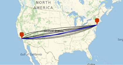
Finally, I wanted to see multiple flight paths on the same map to gain a better understanding of the differences between them. By plotting multiple paths on the same map, I was able to compare them side-by-side. This allowed me to identify the most efficient and effective routes, and to gain a deeper understanding of the trade-offs between different path options.
I used the function below to generate a map of all the paths. This function is similar to findBestPath, except that it plots all the other paths in black by deleting the best path and then individually plotting the best path in a different color. This was one of my favorite parts of the project - It was a blast to see the maps side-by-side and comparing the different routes.
Generates a map with multiple randomly generated paths.
In[]:=
allPaths[leave_,land_]:=Module[{allPath,times,splineList,newSplineList,plotSplines,bestTime,bestIndex,bestPath,randomMap},allPath=Table[pathPlotter[leave,land],{10}];splineList=allPath[[All,2]];times=allPath[[All,1]];bestTime=Min[times];bestIndex=FirstPosition[times,bestTime][[1]];bestPath=splineList[[bestIndex]];newSplineList=Delete[splineList,bestIndex];plotSplines=Partition[Flatten[Table[Table[newSplineList[[x]][y],{y,0,1,0.01}],{x,1,9}]],2];randomMap=GeoGraphics[{{Black,GeoPath[plotSplines]},{Thick,Blue,GeoPath[Table[bestPath[x],{x,0,1,0.01}]]},{Red,GeoMarker[leave]},{Red,GeoMarker[land]}},GeoRange->Entity["Country","UnitedStates"]];randomMap]allPaths,
Out[]=
Conclusion and Future Directions
Conclusion and Future Directions
Overall, I am incredibly pleased with how my project turned out. Through this experience, I was able to deepen my understanding of the Wolfram language and its capabilities. One of the most exciting parts of the project was integrating physics principles with visualizations. While my project operates on the principle that everything is relative, it does have certain limitations. For example, it does not account for factors such as air resistance and lateral movement of the plane caused by wind. This shows that while the flight paths are accurate within the scope’s parameters, they may not reflect all real-world conditions. Despite this, the project still provides valuable insights on the effect of wind on an aircraft. Some further steps with this project would be incorporating more factors into the simulation, developing an app for a streamline approach for flight planning, and creating more flight paths relative to other planes.
Acknowledgements
Acknowledgements
First, thank you to my mentor, Karan, for all the help that he’s given me throughout my project. From explaining concepts to troubleshooting issues, he has been a crucial support for the completion of this project. I also want to extend my heartfelt thanks to Zoya, Alisa, and Nora for their kindness and their assistance with my project and experience. I’m also grateful to the team that has made a foundation for my project and the program- Adam, Meghan, Eryn, and Rory. And a special shout-out to Stephen Wolfram, whose guidance helped me discover a passion project that has been a game-changer for my knowledge.
And finally, thank you to Eric Mason, for inspiring my passion for aviation and aeronautics.
And finally, thank you to Eric Mason, for inspiring my passion for aviation and aeronautics.
Citations
Citations
◼
Frank D and Nykamp DQ, “An introduction to vectors.” From Math Insight. http://mathinsight.org/vector_introduction
◼
Helmenstine, T. (2019, January 29). AP Physics Study Sheet. Science Notes and Projects. https://sciencenotes.org/ap-physics-study-sheet/
◼
Kumari, R. (2024, February 11). Why Airplanes Take Curvy Paths. Medium; Medium. https://medium.com/@rakshakumari090/ever-wondered-why-airplanes-take-curvy-paths-in-the-sky-0b48a9539083
◼
Lange, C. (2021, March 10). Changing style of lines in GeoGraphics. Mathematica Stack Exchange. https://mathematica.stackexchange.com/questions/241530/changing-style-of-lines-in-geographics
◼
Weisstein, Eric W. “Vector Addition.” From MathWorld--A Wolfram Web Resource. https://mathworld.wolfram.com/VectorAddition.html
◼
Wolfram|Alpha Examples: Vectors. (n.d.). www.wolframalpha.com. Retrieved July 10, 2024, from https://www.wolframalpha.com/examples/mathematics/linear-algebra/vectors/
◼
Wolfram, S. (2017, November 14). What Is a Computational Essay?—Stephen Wolfram Writings. Writings.stephenwolfram.com. https://writings.stephenwolfram.com/2017/11/what-is-a-computational-essay/
◼
Wolfram, S., & Wolfram Institute . (1988, June 23). Wolfram Language & System Documentation Center. Reference.wolfram.com; Wolfram Institute . https://reference.wolfram.com/language
CITE THIS NOTEBOOK
CITE THIS NOTEBOOK
Optimizing flight paths for wind
by Abigail Merchant
Wolfram Community, STAFF PICKS, July 12, 2024
https://community.wolfram.com/groups/-/m/t/3215936
by Abigail Merchant
Wolfram Community, STAFF PICKS, July 12, 2024
https://community.wolfram.com/groups/-/m/t/3215936