Originally posted on MSE
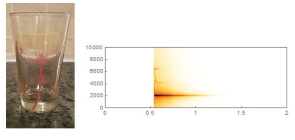
Take an empty glass, hit the side, the glass will make a sound that can be recorded using
s0=AudioCapture["C:\\Users\\...\\Desktop\\\\glass0.wav",MaxDuration->2]
Find the sound spectrum
Spectrogram[s0]
The photo shows a glass and a spectrum of sound
Now we measure the dimensions of the glass, take the density, Young’s modulus, glass Poisson’s ratio from the reference book, compose the equations and find the eigenvalues
<<NDSolve`FEM`;L=.14;L1=.01;r1=.085/2;r2=.055/2;del=.006;(*cg=3962m/s,3980,5100,5640*);
reg=RegionUnion[ImplicitRegion[(r2+(r1-r2)(z-L1)/(L-L1))^2<=x^2+y^2<=(r2+(r1-r2)(z-L1)/(L-L1)+del)^2&&L1<=z<=L,{x,y,z}],ImplicitRegion[0<=x^2+y^2<=(r2+del)^2&&0<=z<=L1,{x,y,z}]];param={Y->56*10^9,ν->25/100};rho=2500;
ClearAll[stressOperator];stressOperator[Y_,ν_]:={Inactive[Div][{{0,0,-((Y*ν)/((1-2*ν)*(1+ν)))},{0,0,0},{-Y/(2*(1+ν)),0,0}}.Inactive[Grad][w[t,x,y,z],{x,y,z}],{x,y,z}]+Inactive[Div][{{0,-((Y*ν)/((1-2*ν)*(1+ν))),0},{-Y/(2*(1+ν)),0,0},{0,0,0}}.Inactive[Grad][v[t,x,y,z],{x,y,z}],{x,y,z}]+Inactive[Div][{{-((Y*(1-ν))/((1-2*ν)*(1+ν))),0,0},{0,-Y/(2*(1+ν)),0},{0,0,-Y/(2*(1+ν))}}.Inactive[Grad][u[t,x,y,z],{x,y,z}],{x,y,z}],Inactive[Div][{{0,0,0},{0,0,-((Y*ν)/((1-2*ν)*(1+ν)))},{0,-Y/(2*(1+ν)),0}}.Inactive[Grad][w[t,x,y,z],{x,y,z}],{x,y,z}]+Inactive[Div][{{0,-Y/(2*(1+ν)),0},{-((Y*ν)/((1-2*ν)*(1+ν))),0,0},{0,0,0}}.Inactive[Grad][u[t,x,y,z],{x,y,z}],{x,y,z}]+Inactive[Div][{{-Y/(2*(1+ν)),0,0},{0,-((Y*(1-ν))/((1-2*ν)*(1+ν))),0},{0,0,-Y/(2*(1+ν))}}.Inactive[Grad][v[t,x,y,z],{x,y,z}],{x,y,z}],Inactive[Div][{{0,0,0},{0,0,-Y/(2*(1+ν))},{0,-((Y*ν)/((1-2*ν)*(1+ν))),0}}.Inactive[Grad][v[t,x,y,z],{x,y,z}],{x,y,z}]+Inactive[Div][{{0,0,-Y/(2*(1+ν))},{0,0,0},{-((Y*ν)/((1-2*ν)*(1+ν))),0,0}}.Inactive[Grad][u[t,x,y,z],{x,y,z}],{x,y,z}]+Inactive[Div][{{-Y/(2*(1+ν)),0,0},{0,-Y/(2*(1+ν)),0},{0,0,-((Y*(1-ν))/((1-2*ν)*(1+ν)))}}.Inactive[Grad][w[t,x,y,z],{x,y,z}],{x,y,z}]};
{vals,funs}=NDEigensystem[stressOperator[56*10^9,1/4]+rho{D[u[t,x,y,z],{t,2}],D[v[t,x,y,z],{t,2}],D[w[t,x,y,z],{t,2}]}=={0,0,0},{u,v,w},t,{x,y,z}∈reg,15];
Frequencies in Hertz
Abs[vals]/(2Pi)
{0.000389602,0.000865814,0.000865814,0.000921462,0.000921462,0.00136215,0.00136215,0.00152256,0.00152256,0.0015598,0.0015598,2140.67,2140.67,2144.36,2144.36}
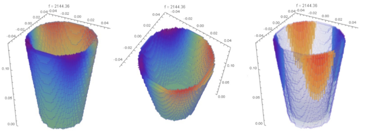
And so we see that frequencies 2140-2144 explain the result of our experiment (in the spectrogram, the peak is about 2000 H). Build 3D functions for frequency 2144.36
u,v,w
DensityPlot3D[Re[funs[[15,1]][x,y,z]],{x,y,z}∈reg,ColorFunction->"Rainbow",OpacityFunction->None,Boxed->False,PlotLabel->Row[{"f = ",Abs[vals[[15]]]/2/Pi}],BoxRatios->Automatic,PlotPoints->50]
DensityPlot3D[Re[funs[[15,2]][x,y,z]],{x,y,z}∈reg,ColorFunction->"Rainbow",OpacityFunction->None,Boxed->False,PlotLabel->Row[{"f = ",Abs[vals[[15]]]/2/Pi}],BoxRatios->Automatic,PlotPoints->50]DensityPlot3D[Re[funs[[15,3]][x,y,z]],{x,y,z}∈reg,ColorFunction->"Rainbow",Boxed->False,PlotLabel->Row[{"f = ",Abs[vals[[15]]]/2/Pi}],BoxRatios->Automatic,PlotPoints->50]
OK! Problems arise if we put del=0.003 (real glass wall thickness). First, the desired frequencies 2140-2144H disappear. Secondly, the 3D functions u,v,w look as if there are holes in the glass
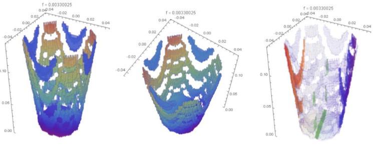
Is it possible to get the desired result for ?
del=.003
Update 1. We use the algorithm proposed by user21 with a small modification and with the boundary condition.
DirichletCondition[{u[t,x,y,z]==0,v[t,x,y,z]==0,w[t,x,y,z]==0},z==0]
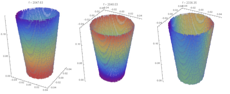
Then the first 5 modes are consistent with the experiment (15 modes can be calculated with an error):
<<NDSolve`FEM`;L=0.14;L1=0.01;r1=0.085/2;r2=0.055/2;del=0.003;
reg=RegionUnion[ImplicitRegion[(r2+(r1-r2)(z-L1)/(L-L1))^2<=x^2+y^2<=(r2+(r1-r2)(z-L1)/(L-L1)+del)^2&&L1<=z<=L,{x,y,z}],ImplicitRegion[0<=x^2+y^2<=(r2+del)^2&&0<=z<=L1,{x,y,z}]];(mesh=ToElementMesh[reg,"BoundaryMeshGenerator"->{"BoundaryDiscretizeRegion",Method->{"MarchingCubes",PlotPoints->31}},"MeshOrder"->1])["Wireframe"]
Modes
{vals,funs}=NDEigensystem[{stressOperator[56*10^9,1/4]+rho{D[u[t,x,y,z],{t,2}],D[v[t,x,y,z],{t,2}],D[w[t,x,y,z],{t,2}]}=={0,0,0},DirichletCondition[{u[t,x,y,z]==0,v[t,x,y,z]==0,w[t,x,y,z]==0},z==0]},{u,v,w},t,{x,y,z}∈mesh,5];
Modes in Hz
Abs[vals]/(2Pi)
{2047.63,2048.03,2048.03,2336.35,2336.35}
There are radial and azimuthal modes
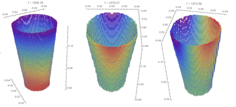
Update 2. We use the algorithm proposed by Pinti with a modification and with the boundary condition.
DirichletCondition[{u[t,x,y,z]==0,v[t,x,y,z]==0,w[t,x,y,z]==0},y==0]
Then the first 9 modes are consistent with the experiment (modes can be calculated without an error):
Get["MeshTools`"]
L=0.14;L1=0.01;r1=0.085/2;r2=0.055/2;del=0.003;
n1=5;n2=31;n3=5;n4=12;mesh2D=StructuredMesh[{{{r2,0},{r1,L}},{{r2-del,0},{r1-del,L}}},{n2,n1}]
mesh2D["Wireframe"[Axes->True,AxesOrigin->{0,0}]]
Modes
{vals,funs}=NDEigensystem[{stressOperator[56*10^9,1/4]+rho{D[u[t,x,y,z],{t,2}],D[v[t,x,y,z],{t,2}],D[w[t,x,y,z],{t,2}]}=={0,0,0},DirichletCondition[{u[t,x,y,z]==0,v[t,x,y,z]==0,w[t,x,y,z]==0},y==0]},{u,v,w},t,{x,y,z}∈mesh,9];
vals in Hz
Abs[vals]/(2Pi)
{23.1411,1806.36,1806.36,1806.36,1806.36,1970.47,1970.47,1970.58,1970.58}
There are radial and azimuthal modes too
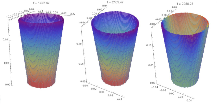
Update 3. We use the algorithm proposed by user21 for version 12.1 with a small modification
<<NDSolve`FEM`;L=0.14;L1=0.01;del=0.003;r1=0.085/2;r2=0.055/2;
polygon=Polygon[{{0,0,0},{r2+del,0,0},{r2+del,0,L1},{r1+del,0,L},{r1,0,L},{r2,0,L1},{0,0,L1}}];
Needs["OpenCascadeLink`"]shape=OpenCascadeShape[polygon];axis={{0,0,0},{0,0,3/2L}};sweep=OpenCascadeShapeRotationalSweep[shape,axis,2Pi];bmesh=OpenCascadeShapeSurfaceMeshToBoundaryMesh[sweep,"ShapeSurfaceMeshOptions"->{"LinearDeflection"->0.0003}];
mesh=ToElementMesh[bmesh,AccuracyGoal->5,PrecisionGoal->5,"MeshOrder"->1];
param={Y->56*10^9,ν->25/100};rho=2500;cg=Sqrt[56.*10^9/rho];
ClearAll[stressOperator];stressOperator[Y_,ν_]:={Inactive[Div][{{0,0,-((Y*ν)/((1-2*ν)*(1+ν)))},{0,0,0},{-Y/(2*(1+ν)),0,0}}.Inactive[Grad][w[t,x,y,z],{x,y,z}],{x,y,z}]+Inactive[Div][{{0,-((Y*ν)/((1-2*ν)*(1+ν))),0},{-Y/(2*(1+ν)),0,0},{0,0,0}}.Inactive[Grad][v[t,x,y,z],{x,y,z}],{x,y,z}]+Inactive[Div][{{-((Y*(1-ν))/((1-2*ν)*(1+ν))),0,0},{0,-Y/(2*(1+ν)),0},{0,0,-Y/(2*(1+ν))}}.Inactive[Grad][u[t,x,y,z],{x,y,z}],{x,y,z}],Inactive[Div][{{0,0,0},{0,0,-((Y*ν)/((1-2*ν)*(1+ν)))},{0,-Y/(2*(1+ν)),0}}.Inactive[Grad][w[t,x,y,z],{x,y,z}],{x,y,z}]+Inactive[Div][{{0,-Y/(2*(1+ν)),0},{-((Y*ν)/((1-2*ν)*(1+ν))),0,0},{0,0,0}}.Inactive[Grad][u[t,x,y,z],{x,y,z}],{x,y,z}]+Inactive[Div][{{-Y/(2*(1+ν)),0,0},{0,-((Y*(1-ν))/((1-2*ν)*(1+ν))),0},{0,0,-Y/(2*(1+ν))}}.Inactive[Grad][v[t,x,y,z],{x,y,z}],{x,y,z}],Inactive[Div][{{0,0,0},{0,0,-Y/(2*(1+ν))},{0,-((Y*ν)/((1-2*ν)*(1+ν))),0}}.Inactive[Grad][v[t,x,y,z],{x,y,z}],{x,y,z}]+Inactive[Div][{{0,0,-Y/(2*(1+ν))},{0,0,0},{-((Y*ν)/((1-2*ν)*(1+ν))),0,0}}.Inactive[Grad][u[t,x,y,z],{x,y,z}],{x,y,z}]+Inactive[Div][{{-Y/(2*(1+ν)),0,0},{0,-Y/(2*(1+ν)),0},{0,0,-((Y*(1-ν))/((1-2*ν)*(1+ν)))}}.Inactive[Grad][w[t,x,y,z],{x,y,z}],{x,y,z}]};
{vals,funs}=NDEigensystem[{stressOperator[56*10^9,1/4]+rho{D[u[t,x,y,z],{t,2}],D[v[t,x,y,z],{t,2}],D[w[t,x,y,z],{t,2}]}=={0,0,0},DirichletCondition[{u[t,x,y,z]==0,v[t,x,y,z]==0,w[t,x,y,z]==0},z==0]},{u,v,w},t,{x,y,z}∈mesh,12];
vals in Hz
Abs[vals]/(2Pi)
{1973.97,1973.97,1974.86,1974.86,2169.47,2169.47,2250.23,2250.23,4183.69,4183.69,5532.12,5532.12}
Visualisation of 3 modes
DensityPlot3D[Re[funs[[1,1]][x,y,z]],{x,y,z}∈mesh,ColorFunction->"Rainbow",OpacityFunction->None,Boxed->False,PlotLabel->Row[{"f = ",Abs[vals[[1]]]/2/Pi}],BoxRatios->Automatic,PlotPoints->50]DensityPlot3D[Re[funs[[5,1]][x,y,z]],{x,y,z}∈mesh,ColorFunction->"Rainbow",OpacityFunction->None,Boxed->False,PlotLabel->Row[{"f = ",Abs[vals[[5]]]/2/Pi}],BoxRatios->Automatic,PlotPoints->50]DensityPlot3D[Re[funs[[7,1]][x,y,z]],{x,y,z}∈mesh,ColorFunction->"Rainbow",OpacityFunction->None,Boxed->False,PlotLabel->Row[{"f = ",Abs[vals[[7]]]/2/Pi}],BoxRatios->Automatic,PlotPoints->50]
CITE THIS NOTEBOOK
CITE THIS NOTEBOOK
3D elastic waves in a drinking glass: radial and azimuthal mode analysis, FEM, Dirichlet conditions
by Alexander Trounev
Wolfram Community, STAFF PICKS, October 9, 2024
https://community.wolfram.com/groups/-/m/t/3295343
by Alexander Trounev
Wolfram Community, STAFF PICKS, October 9, 2024
https://community.wolfram.com/groups/-/m/t/3295343