Additional examples for the first discussion
Give DALL.E a piece of WL code that produces a graphics and that is not straightforward to predict in detail. It is interesting (and entertaining) to see how it ‘understands’ the code and predicts what the result could look like.
DALL·E 2 prompt
DALL·E 2 prompt
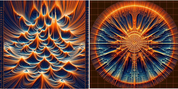
Analyze the following code carefully and make an artistic rendering of how you think the result would look like:
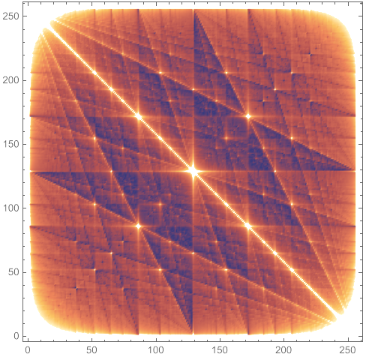
The Wolfram Language input code and its output graphics
The Wolfram Language input code and its output graphics
ListDensityPlot[Abs[Fourier[Table[1/LCM[i,j],{i,256},{j,256}]]],Mesh->False]
DALL-E AI prediction from reading the input code
DALL-E AI prediction from reading the input code
The Wolfram Language input code and its output graphics
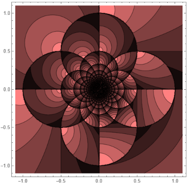
The Wolfram Language input code and its output graphics
In[]:=
ContourPlotAbs[1/(x+Iy)-Floor[1/(x+Iy)]], {x,-1.1,1.1},{y,-1.1,1.1},Exclusions->None,PlotPoints->50,ColorFunction->Function[Blend[{Pink,Black},#]]
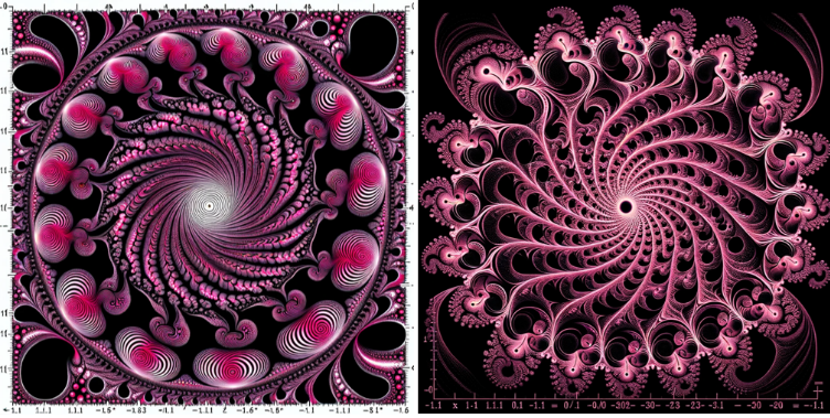
DALL-E AI prediction from reading the input code
DALL-E AI prediction from reading the input code
The Wolfram Language input code and its output graphics
The Wolfram Language input code and its output graphics
In[]:=
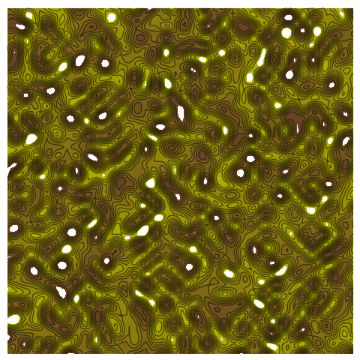
ListContourPlot[Table[Random[],{36},{36}],ColorFunction->Function[Blend[{Darker[Yellow],Darker[Brown]},#]],InterpolationOrder->4,Frame->False]
Out[]=
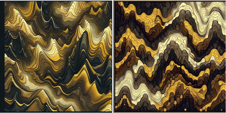
DALL-E AI prediction from reading the input code
DALL-E AI prediction from reading the input code
The Wolfram Language input code and its output graphics
The Wolfram Language input code and its output graphics
In[]:=
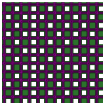
ListContourPlot[Table[If[EvenQ[#],1,0]&[(n+m)(n-m+1)/2],{n,25},{m,25}],ColorFunction->Function[Blend[{Purple,Darker[Green]},(Cos[2Pi#]+1)/3]],InterpolationOrder->1,Frame->False,PlotRange->All]
Out[]=
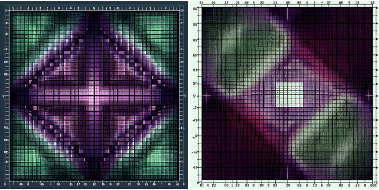
DALL-E AI prediction from reading the input code
DALL-E AI prediction from reading the input code
The Wolfram Language input code and its output graphics
The Wolfram Language input code and its output graphics
In[]:=
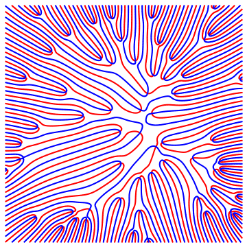
ContourPlot[Evaluate[(#==0)&/@ReIm[Product[(x+Iy)-(RandomReal[]+IRandomReal[]),{60}]]],{x,0,1},{y,0,1},(*usemanyplotpointstoachievehighresolution*)PlotPoints->100,PlotRange->All,FrameTicks->None,Frame->False,ContourStyle->{Red,Blue}]
Out[]=
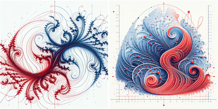
DALL-E AI prediction from reading the input code
DALL-E AI prediction from reading the input code
The Wolfram Language input code and its output graphics
The Wolfram Language input code and its output graphics
In[]:=
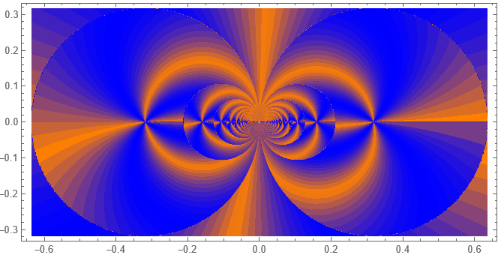
ContourPlot[Arg[ArcTan[Tan[(x+Iy)^(-1)]]],{x,-2/Pi,2/Pi},{y,-1/Pi,1/Pi},PlotPoints->100,ContourLines->False,Exclusions->None,PlotRange->All,ColorFunction->Function[Blend[{Orange,Blue},Abs[Sin[12#]]]],AspectRatio->Automatic,Contours->100]
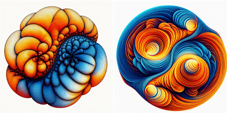
DALL-E AI prediction from reading the input code
DALL-E AI prediction from reading the input code
The Wolfram Language input code and its output graphics
The Wolfram Language input code and its output graphics
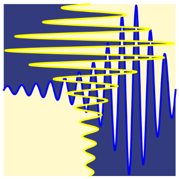
intersectionPicture[δ_,opts___]:=Show[{(*thecontourplot*)ContourPlot[(y-Pi/((x-δ)^2+1)Sin[12(x-δ)])(x-Pi/((y-δ)^2+1)Sin[12(y-δ)]),{x,-Pi,Pi},{y,-Pi,Pi},PlotPoints->100,Contours->{0},ContourLines->False,PlotRange->All,FrameTicks->None],(*y=y(x)curve*)ParametricPlot[{x,Pi/((x-δ)^2+1)Sin[12(x-δ)]},{x,-Pi,Pi},PlotRange->All,PlotPoints->100,PlotStyle->{Blue,Thickness[0.01]}],(*x=x(y)curve*)ParametricPlot[{Pi/((x-δ)^2+1)Sin[12(x-δ)],x},{x,-Pi,Pi},PlotRange->All,PlotPoints->100,PlotStyle->{Yellow,Thickness[0.01]}]},opts,Frame->False];intersectionPicture[Pi/2]
Out[]=
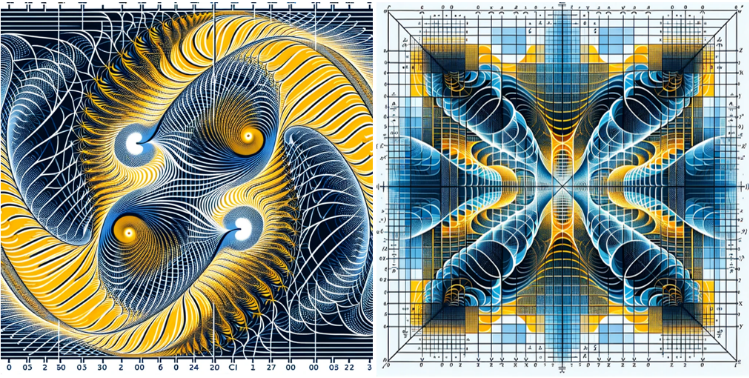
DALL-E AI prediction from reading the input code
DALL-E AI prediction from reading the input code
The Wolfram Language input code and its output graphics
The Wolfram Language input code and its output graphics
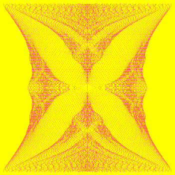
With[{n=14},Module[{M,α},(*matrixtobediagonalizedforvariousΦ*)Set@@{M[α_],N[makeLhsMatrix[n,Φ]]};(*showgraphicofeigenvalues*)Graphics[{Thickness[0.002],PointSize[0.003],Lighter[Red],(*mirroratΦ=1/2*){#,Apply[{#1,1-#2}&,#,{-2}]}&[Line/@Transpose[Table[Re[{#,Φ}]&/@Sort[Eigenvalues[M[Φ]]],{Φ,0.,1/2.,1/2./(n-1)^2}]]]}/.(*forbettervisibilityonscreen*)Line[l_]:>Point/@l,AspectRatio->1,Background->Yellow,PlotRange->All]]]
Out[]=
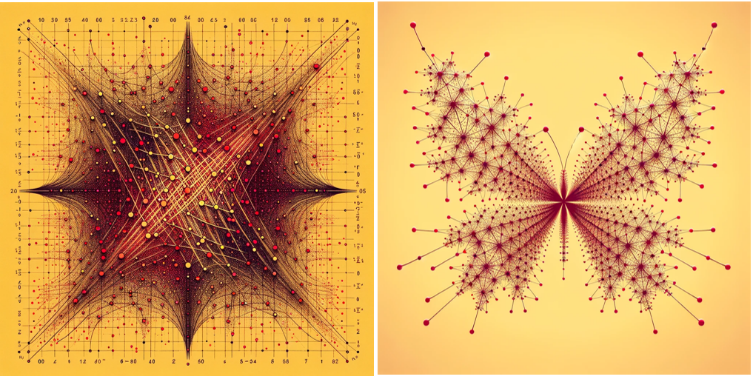
DALL-E AI prediction from reading the input code
DALL-E AI prediction from reading the input code
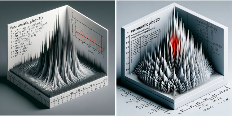
The Wolfram Language input code and its output graphics
The Wolfram Language input code and its output graphics
{ℋ0,ℋ1}=With[{n=12},Table[(#1+Transpose[#1]&)[Table[If[i>j,0.,2Random[]-1],{i,n},{j,n}]],{2}]];minEigenvalueDistance[ℋ_?MatrixQ]:=Module[{evs=Eigenvalues[ℋ],n=Length[ℋ]},Min[Table[Min[Table[Abs[evs〚i〛-evs〚j〛],{j,i+1,n}]],{i,1,n-1}]]]ParametricPlot3D[{αrCos[αφ],αrSin[αφ],-Log[minEigenvalueDistance[N[(1-αrExp[αφ])ℋ0+αrExp[αφ]ℋ1]]]},{αr,0,2.5},{αφ,0,2π},BoxRatios{1,1,0.6},PlotRange{All,All,{-1,5}},PlotStyle->Directive[GrayLevel[0.3],Specularity[Red,10]],Mesh->None]
Out[]=

DALL-E AI prediction from reading the input code
DALL-E AI prediction from reading the input code
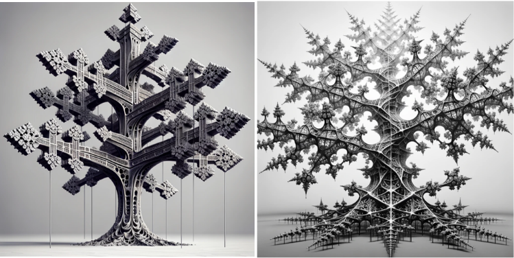
The Wolfram Language input code and its output graphics
The Wolfram Language input code and its output graphics
(*makeoneelementarypartofthesignpost*)post[α_,dir_,ortho_,size_]:=Module[{dir1,orthoh,ortho1,bi,p1,p2,p3,p4,p5,p6,p7,p8,p9,s1=1,s2=0.3,s3=0.2,s4=1.2,h1,h2,h3,h4,h5},(*directionthenewsignwillpointto*)dir1=Normalize[dir];(*firstorthogonaldirection*)ortho1=Normalize[Normalize[ortho]+Normalize[Cross[dir,ortho]]];(*secondorthogonaldirection*)bi=Normalize[Cross[dir1,ortho1]];h1=s2sizeortho1;h2=s2sizebi;h3=s3sizeortho1;h4=s3sizebi;h5=s1sizedir1;p1=α+h1;p2=α+h2;p3=α-h1;p4=α-h2;p5=α+h3+h5;p6=α+h4+h5;p7=α-h3+h5;p8=α-h4+h5;p9=α+s4sizedir1;(*polygonsformingthenextgeneration*)Polygon/@{{p1,p4,p8,p5},{p4,p3,p7,p8},{p3,p2,p6,p7},{p2,p1,p5,p6},{p5,p9,p8},{p8,p7,p9},{p6,p7,p9},{p5,p6,p9}}](*thestartpart*)postHierarchy[0]={post[{0.,0.,0.},{0.,0.,1.},{1.,0.,0.},1]};(*addnewpartsatthesides*)postHierarchy[i_]:=postHierarchy[i]=(post@@newData[#,0.4^i])&/@Flatten[(Take[#,4]&/@postHierarchy[i-1])];(*iteratetheprocess*)newData[poly_Polygon,size_]:=Module[{f=poly[[1]],ortho,dir,p},ortho=(f[[1]]+f[[2]])/2-(f[[3]]+f[[4]])/2;p=(f[[3]]+f[[4]])/2+0.2ortho;dir=-Cross[f[[1]]-f[[2]],f[[1]]-f[[4]]];{p,dir,ortho,size}]
In[]:=
Show[Graphics3D[{EdgeForm[Thickness[0.001]],Table[postHierarchy[i],{i,0,4}]}]]
Out[]=

DALL-E AI prediction from reading the input code
DALL-E AI prediction from reading the input code
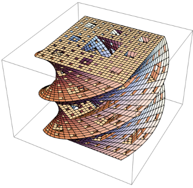
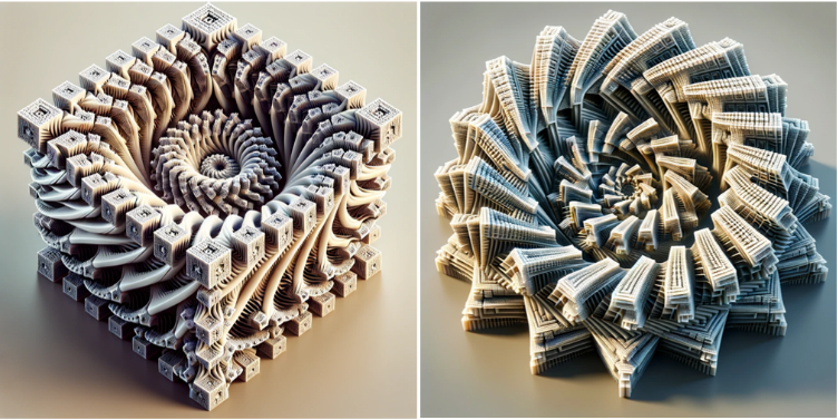
The Wolfram Language input code and its output graphics
The Wolfram Language input code and its output graphics
polys=Map[2(#-1/2)&,MeshPrimitives[MengerMesh[3,3],{2}],{-2}];twist[{x_,y_,z_}]:=RotationTransform[Pi/2z,{0,0,1}][{x,y,z}];twist[Polygon[l_]]:=Polygon[twist/@l]Graphics3D[twist/@polys]
DALL-E AI prediction from reading the input code
DALL-E AI prediction from reading the input code
CITE THIS NOTEBOOK
CITE THIS NOTEBOOK
DALL-E AI artistic renderings predicted from graphics-generating code: Part II
by Michael Trott
Wolfram Community, STAFF PICKS, January 29, 2024
https://community.wolfram.com/groups/-/m/t/3112314
by Michael Trott
Wolfram Community, STAFF PICKS, January 29, 2024
https://community.wolfram.com/groups/-/m/t/3112314