0. abstract
0. abstract
Every M. C. Escher’s work is a math and visual puzzle for his enthusiasts. Many Escher’s works have been well explained with math concepts, like 2D tessellation, loxodromic spirals, hyperbolic geometry, conformal isomorphism, etc.
In the article, authors are going to explain how we analysis Escher’s work (Cubic space division, 1952) based by linear perspective, then we reconstruct a 3D cubics lattice model to re-produce a Escher’s style 2D image. Escher’s related work, methods and techniques will be discussed in details.
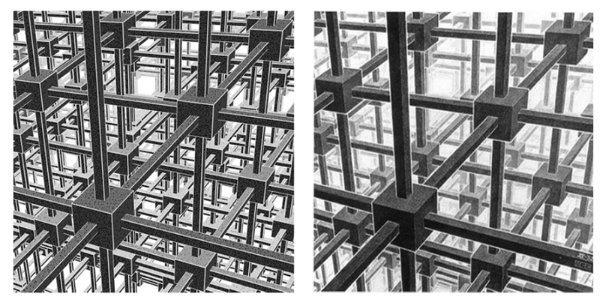
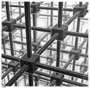
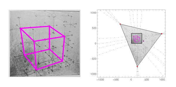
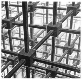
Compare the following two images. Can you tell which one is Escher’s original work?
1. background
1. background
1.0 initializing
1.0 initializing
1.1 perspective in painting
1.1 perspective in painting
Perspective originated in the field of painting, where people pondered and tried to solve the question: “How to represents 3D objects in space on a 2D canvas, realistically? In the meanwhile, it need to conform to visual experience of human eyes.” The earliest Greeks or Romans may have mastered single-point perspective, but this technique was lost. Fortunately, thanks to the appreciation and promotion from Leonardo da Vinci and Dürer, perspective once again became the core theory of painting in the Renaissance.
1.1.1 single-point perspective
1.1.1 single-point perspective
In single-point perspective, there is only one vanishing point, which is identical to the principal point located on the horizon line. In single-point perspective, for a 3D object of a box, the front of the box will be parallel to the image plane or canvas plane. Vanishing points can be found by converging the extension lines of a box or rectangular edge in the frame. Single-point perspective in photography or painting is often used to represent endless stretches of roads or railroad tracks, but it can also be a good representation of the depth of field of indoor scenes, such as Leonardo da Vinci’s famous work “The Last Supper” is a good example. The vanishing point are located just to the left of the face of the central figure Jesus.
Out[]=
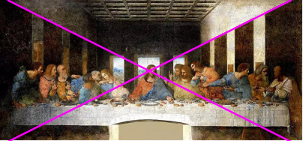
Source : Leonardo da Vinci, The Last Supper, 1494-1498.
1.1.2 two-point perspective
1.1.2 two-point perspective
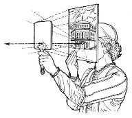
A two-point perspective has two vanishing points, usually the line between the two vanishing points is the horizon line, and the principal point is centered at the midpoint of the two vanishing points. In two-point perspective for a 3D object of a box, the vertical edge of the box will be perpendicular to the horizon line, while the front of the box will be rotated along the Z-direction at an certain angle, the front and sides will be both displayed. The vanishing points can be found by converging the extension line of the box or rectangular edge in the picture. Two-point perspective represents street scenes or architecture with good third-dimensional sense. The first building in history to be painted precisely according to two-point perspective was the Florentine Baptistery in the fifteenth century, which happened to be an octagonal building. The painter Filippo Brunelleschi also designed a double-sided reflecting mirror to verify that his work is exactly the same as the actual building.
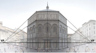
Source : Filippo Brunelleschi, Florentine Baptistery (octagonal building), 15th Century
1.1.3 three-point perspective
1.1.3 three-point perspective
Three-point perspective has three vanishing points, and the connection of the three vanishing points is called the vanishing line. Three-point perspective is a general linear perspective model that no longer requires any specific constraint (parallel or vertical) between the object and viewer. In other words, the 3D view box can be placed in any position or orientation. In painting and photography, three-point perspective are used to represent the height of buildings and skyscrapers, such as bird’s eye or ant’s eye view. If it is a bird’s eye view, the third vanishing point is called nadirs. If it is an ant’s eye view, it is called zeniths.
Three-point perspective is frequently involved in Escher’s work, such as one of his early works, Tower of Babel. Edges on both sides of the building intersect to form two vanishing points in the direction of the horizon similar to two-point perspective. At the same time, unlike the two-point perspective, the vertical boundary line will intersect to form a third vanishing point. This downward intersection of vertical boundaries creates a strong sense of vertical perspective at the nadir, which highlights the building’s unbelievable height.
Out[]=
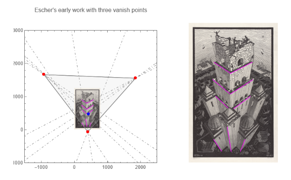
Source: M. C. Escher, Tower of Babel, 1928.
1.2 perspective in computer graphics
1.2 perspective in computer graphics
Entering the information age and the rapid development of computers and software, linear perspective has been applied to computer graphics. In computer graphics, perspective is commonly regarded as pinhole model, its process and method as shown in the following figure.
It should be pointed out that perspective projection in computer graphics is actually solving the same problem as traditional perspective painting, how to correctly project 3D objects onto a 2D image plane or screen. The difference is that the computer graphics uses mathematics, geometry and algorithms to describe the perspective projection relationship. The process is more automatic, and the result is more precise.
1.3 perspective of simple RGB cubic
1.3 perspective of simple RGB cubic
Let’s build a Wolfram demo project to better understand linear perspective.
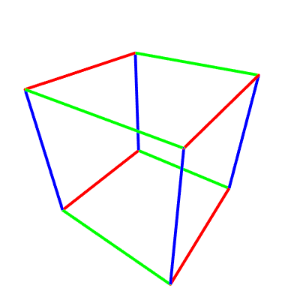
First, we build an RGB cube with red on X-direction edge, green on the Y-direction edge, and blue on the Z-direction edge.
In[]:=
xlines={{{1,1,1},{-1,1,1}},{{1,-1,1},{-1,-1,1}},{{1,-1,-1},{-1,-1,-1}},{{1,1,-1},{-1,1,-1}}};ylines={{{1,1,1},{1,-1,1}},{{-1,1,1},{-1,-1,1}},{{-1,1,-1},{-1,-1,-1}},{{1,1,-1},{1,-1,-1}}};zlines={{{1,1,1},{1,1,-1}},{{-1,1,1},{-1,1,-1}},{{-1,-1,1},{-1,-1,-1}},{{1,-1,1},{1,-1,-1}}};
In[]:=
img=Image@Graphics3D[{Thickness[0.01],RGBColor[1,0,0],Line/@xlines,RGBColor[0,1,0],Line/@ylines,RGBColor[0,0,1],Line/@zlines},ImageSize->400,ViewVector->{2{1,1,1}//RotationTransform[-10Degree,{0,0,1}],{0,0,0}},Boxed->False,ImagePadding10]
Out[]=
Due to the difference in color of their three directional edges, we can easily track and calculate the vanishing point of the cube and the orthocenter of the vanishing triangle.
In[]:=
bounds2D={{0,0},ImageDimensions[img]};{r,g,b}=ColorSeparate[img];lineImage={ImageSubtract[img,g,b],ImageSubtract[img,r,b],ImageSubtract[img,r,g]};lines=ImageLines[EdgeDetect[#],0.1]&/@lineImage;linePrts=Map[First,lines,{2}];viewLines=Subsets[#,{2}]&/@linePrts;intersectionPrts=Select[#,ListQ[#]&]&/@Map[LineIntersection,viewLines,{2}];intersectionPrts=If[Length[#]==0,{{10^6,10^6}},#]&/@intersectionPrts;vanishPrts=Mean/@intersectionPrts;orthocenter=TriangleCenter[vanishPrts,"Orthocenter"]
Out[]=
{202.286,192.306}
In[]:=
Image[plot=Graphics[{Opacity[0.3],LightGray,EdgeForm[Gray],Polygon[vanishPrts],EdgeForm[{Black,Dashed}],Opacity[0.5],LightGray,Rectangle@@bounds2D,Thickness[0.004],RGBColor[1,0,0],Line/@linePrts[[1]],RGBColor[0,1,0],Line/@linePrts[[2]],RGBColor[0,0,1],Line/@linePrts[[3]],Thickness[0.002],Gray,DotDashed,Map[InfiniteLine,linePrts,{2}],Opacity[1],Red,PointSize[0.02],Point/@vanishPrts,Purple,Point[orthocenter]},PlotRange1000{{-1,1},{-1,1}},Frame->True,ImageSize->300]]
Out[]=
Finally, we put them together. The upper-left view is a view based on the world coordinate system, with a black cube as the target object and red arrows as the direction of view. The upper middle view is the observed RGB cube in the camera coordinate system. The lower-left view is the zoom out view, which contains the vanishing point, the orthocenter of vanishing triangle, and the image boundary. The lower-right table shows the current view options, and the slider on the right controls the view options.
Out[]=


By this computational experimental, it is not difficult to find that three-point perspective is an universal model for linear perspective, while single-point perspective and two-point perspective are a special case with objects and camera under specific constrained conditions.
1. Single-point perspective requires that the front plane of cube is just parallel to image plane, and two vanishing points are actually at infinity.
2. Two-point perspective requires that the vertical direction of object is exactly perpendicular to horizon line of view, and one vanishing point is also at infinity.
3. Three-point perspective does not require any geometric constraints, and all three perspective points can find their position within a limited range。
Combining single-point, two-point, and three-point perspectives together is the full content and view angle of linear perspective.
1.4 Identification of problems
1.4 Identification of problems
To further analyze the problem, we can divide the perspective-related problems into two types.
Forward problem: human eye, painting, cameras, and computer graphics solves the forward problems. In this type of problem, the known or input conditions are the position and orientation of viewer, the geometry and size of the object in 3D, the position and orientation of the object in 3D. It solved and output a correct 2D image that meets all these criteria. The forward problem, from 3D to 2D, is certainty and completion of information, and its solution is unique.
Inverse problem: machine vision or reverse reconstruction solves the inverse problem. In this type of problem, the known or input condition is merely an image of a 2D object, through which the view point or camera position can be estimated or assumed. With some further assumed or identified information, like shape and size of the 3D object. Finally, all the associated information, like position and orientation of 3D object, can obtained as output. The inverse problem, from 2D to 3D, is uncertainty and in-completion of information, and the solution is not unique.
Out[]=
problem | input | output | method / device | |||||
forward problem |
| 2D image |
| |||||
inverse problem | 2D image |
|
|
2. analysis Escher’s work
2. analysis Escher’s work
In this section, we will analyze Escher’s work in detail through the principle of linear perspective with the insight of how Escher created it.
2.1 find view options in 2D
2.1 find view options in 2D
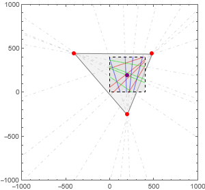
Find vanishing points from the edge lines.
In[]:=
image=ImageResizeImageCrop
,350{1,1};bounds2D={{0,0},ImageDimensions[image]};
In[]:=
lines=ImageLines[EdgeDetect[image],0.22,0.07];h=HighlightImage[image,lines];
Based on the vanishing point, we can further calculate vanishing line, horizon line and principle point.
In[]:=
linePrts=First[#]&/@lines;viewLines=Subsets[linePrts,{2}];intersectionPrts=Select[LineIntersection/@viewLines,ListQ[#]&];lookingPrts={{-1040,400},{800,800},{200,-1000}};intersectionPrtsCorner=Table[Select[intersectionPrts,(EuclideanDistance[#,lookingPrts[[i]]]<=300)&],{i,Length@lookingPrts}];vanishPrts=Mean/@intersectionPrtsCorner
Out[]=
{{-1083.65,410.219},{781.988,800.656},{170.321,-1034.51}}
In[]:=
Row[{Graphics[{Lighter@LightGray,EdgeForm[Gray],Polygon[vanishPrts],Texture[image],Polygon[{{0,0},{350,0},{350,350},{0,350}},VertexTextureCoordinates{{0,0},{1,0},{1,1},{0,1}}],Thickness[0.004],Magenta,lines,EdgeForm[Directive[Thick,Black]],Opacity[0.1],LightGray,Rectangle@@bounds2D,Opacity[1],Thickness[0.002],Gray,DotDashed,InfiniteLine/@linePrts,PointSize[0.01],Blue,Point/@intersectionPrtsCorner,Red,Point/@vanishPrts,Black,Line[{{0.`,251.78831260059732`},{350.`,199.52013084486055`}}]},PlotRange1300{{-1,1},{-1,1}},Frame->True,ImageSize->450,ImagePadding25,PlotLabel->Style["estimate vanishing points position",16,Bold]],Column[Table[Graphics[{Lighter@LightGray,EdgeForm[Gray],Polygon[vanishPrts],Thickness[0.002],Gray,DotDashed,InfiniteLine/@linePrts,PointSize[0.03],Blue,Point/@intersectionPrts,Red,Point/@vanishPrts},PlotRangeTranspose@{vanishPrts[[i]]-100{1,1},vanishPrts[[i]]+100{1,1}},Frame->True,ImageSize->140,ImagePadding20],{i,3}],Alignment->Center,Spacings->1]}]
Out[]=
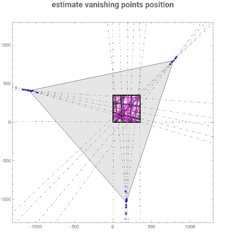
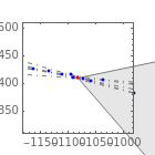
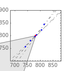
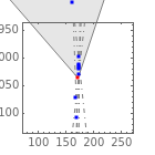
Estimate the location of the vanishing point, the intersection of any two lines is likely to be a vanishing point. We regards the mean points of intersection points as a true vanishing point.
From the calculations here, we can be seen that Escher’s work are very precise. Within the area of 2000 ×2000, the offset of the vanishing points are within 100 along the direction of auxiliary horizon line. This means that the maximum angle error for Escher edge lines is about 0.00027 Rad or 0.015 degree. At Escher’s age, there were no computers and plotters, the available tooling are pens and rulers, and it was not easy to achieve such precise.
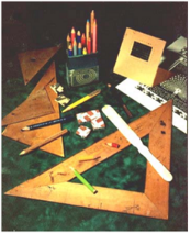
Photograph of objects in M. C. Escher’s Studio
In[]:=
orthocenter=TriangleCenter[vanishPrts,"Orthocenter"]interiorAngle=Table[TriangleMeasurement[vanishPrts,{"InteriorAngle",vanishPrts[[i]]}]*(180/Pi),{i,3}]edgeLength=Norm/@Subsets[vanishPrts,{2}]area=Area[Polygon[vanishPrts]]horizontalLine=Drop[vanishPrts,-1]
Out[]=
{-60.6734,69.2574}
Out[]=
{60.8634,59.7464,59.3902}
Out[]=
{1348.5,1357.15,1369.38}
Out[]=
1.59246×
6
10
Out[]=
{{-1083.65,410.219},{781.988,800.656}}
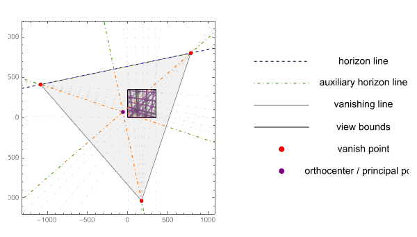
Let’s further visualize the vanishing line, the horizon line, and the principal point. It should be noted, that we later regard the orthocenter of the vanishing triangle to be the principal point of view.
In[]:=
g=Graphics[{Opacity[0.3],Lighter@LightGray,EdgeForm[Gray],Polygon[vanishPrts],Texture[image],Polygon[{{0,0},{350,0},{350,350},{0,350}},VertexTextureCoordinates{{0,0},{1,0},{1,1},{0,1}}],Thickness[0.004],Magenta,lines,EdgeForm[Directive[Thickness[0.004],Black]],Opacity[0.1],LightGray,Rectangle@@bounds2D,Thickness[0.002],Gray,DotDashed,InfiniteLine/@linePrts,Thickness[0.004],Opacity[1],Dashed,Blue,InfiniteLine[horizontalLine],DotDashed,Orange,InfiniteLine[{#,orthocenter}]&/@vanishPrts,Red,PointSize[0.02],Point/@vanishPrts,Purple,Point[orthocenter]},PlotRange1200{{-1.1,0.9},{-1,1}},Frame->True,ImageSize->350,ImagePadding25];
In[]:=
legends=Graphics[{Purple,Disk[{.25,-.1},.025],Black,Style[Text["orthocenter / principal point",{1,-.1}],14],Red,Disk[{.25,.1},.025],Black,Style[Text["vanish point",{1,.1}],14],Thickness[0.004],Black,Line[{{0,.3},{.5,.3}}],Black,Style[Text["view bounds",{1,.3}],14],Gray,Line[{{0,.5},{.5,.5}}],Black,Style[Text["vanishing line",{1,.5}],14],Orange,DotDashed,Line[{{0,.7},{.5,.7}}],Black,Style[Text["auxiliary horizon line",{1,.7}],14],Blue,Dashed,Line[{{0,.9},{.5,.9}}],Black,Style[Text["horizon line",{1,.9}],14]},ImageSize->{250,250},PlotRange->All];
Out[]=
2.2 find direction of view in 3D
2.2 find direction of view in 3D
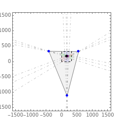
In this section, we move from 2D to 3D. Base on the principal point (orthocenter) of view, we can determinate the view vector. Suppose the image plane is at Z = -500 and parallel to XY plane. The image plane is the projection plane or canvas plane in this case .
In[]:=
iPZ=-500;(*imageplaneZ*)vanishPrts3D=Map[Append[#,iPZ]&,vanishPrts]orthocenter3D=Append[orthocenter,iPZ]bounds3D=Map[Append[#,iPZ+0.1]&,{{0,0},{350,0},{350,350},{0,350}}]
Out[]=
{{-1083.65,410.219,-500},{781.988,800.656,-500},{170.321,-1034.51,-500}}
Out[]=
{-60.6734,69.2574,-500}
Out[]=
{{0,0,-499.9},{350,0,-499.9},{350,350,-499.9},{0,350,-499.9}}
The vector from the view point to the principal point is called the direction of view. In another words, the view point is always located on the center line of view. The center line of view is perpendicular to the image plane. Since the problem we are solving is from 2D to 3D, theoretically the view point can be located at any position in the center line of view, because we do not know the true size of the 3D object and the position of view point. We are just measuring the related scale between the 2D image and the 3D object. For simplification, we assume that the view point is at certain position on the center line of view.
Out[]=
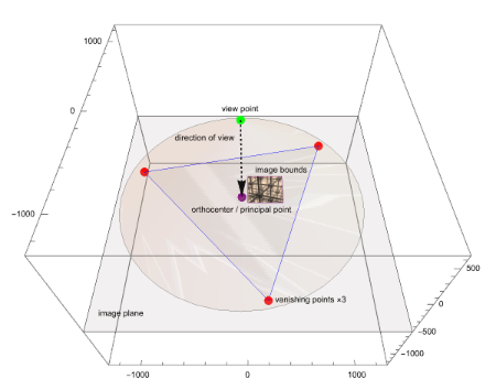
Pay special attention to the detail, the center line of view is located at the outside of view frame or image boundary. Near the lower-left corner of image bounds is the principal point of view in purple. This situation is very uncommon for both traditional art painting and modern computer graphics. In art painting, camera photograph, or computer graphics, the center line of view and principal point will be always enclosed within the view frame or image boundary.
2.3 pick vertices of cube as samples
2.3 pick vertices of cube as samples
When Escher creates a new lithography, it is very likely that he will first draw a draft with a pencil. We didn’t find the exactly draft for his cubic work, but the reference[1] provides another very similar draft. In this draft he marked the 3D coordinate system for main vertices, circled with numbers in the centers, and he also represented proportional relations in space using the length of axis. Interestingly, the perspective of this draft is also that the principal point is located out of the image boundary, but on the right side this time.
Out[]=
Source: M.C. Escher, Preliminary Study for Depth, pencil, 1955.
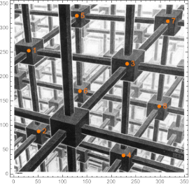
Inspired by Escher’s drafts, and if you look closely at the lithograph, you can find that Escher painted a complete cube. We obtain the 8 vertex coordinates of this cube by sampling on the image. The Mathematica coordinates tool allows for a simple one-time operation to get coordinates on an image.
In[]:=
pickSample={{30.57`,253.33`},{50.76`,87.53`},{232.18`,226.47`},{224.69`,38.07`},{129.02`,325.14`},{135.36`,170.32`},{315.55`,313.98`},{297.97`,139.`}};
In[]:=
Image@Graphics[{Texture[image],Polygon[350{{0,0},{1,0},{1,1},{0,1}},VertexTextureCoordinates{{0,0},{1,0},{1,1},{0,1}}],PointSize[0.02],Orange,Point/@pickSample,MapIndexed[Text[Style[First[#2],14],#1,{-3,0}]&,pickSample]},Axes->True,Frame->True]
Out[]=
2.4 optimizing cubic projection in 3D
2.4 optimizing cubic projection in 3D
Next, we assume that the camera is located at the vertical Z= 260 position. In another words, the view point is at a specific point on the center line of view. The 2D coordinates of 8 vertices of the cube are known on image plane, and 7 unknown variables need to be solved, namely: cube size (edge length) and cube orientation and position (6 DoF), that is, the orientation {α,β,γ} and the position {x0,y0,z0} of cubic center.
In[]:=
Clear[α,β,γ,r,x0,y0,z0]
In[]:=
projection[cP_,n_,iP_][r_]:=cP-(r-cP)*(n.(cP-iP)/n.(r-cP));solid=PolyhedronData["Cube","GraphicsComplex"];edges=PolyhedronData["Cube","EdgeIndices"]*{{1,2},{1,3},{1,5},{2,4},{2,6},{3,4},{3,7},{4,8},{5,6},{5,7},{6,8},{7,8}};cube[{α_,β_,γ_},r_,{x0_,y0_,z0_}]:={solid[[2,1]],(TranslationTransform[{x0,y0,z0}].AffineTransform[{EulerMatrix[{γ,β,α},{1,2,1}],{0,0,0}}].ScalingTransform[{r,r,r}])/@solid[[1]]};
In[]:=
cameraPosition={-56.55423148932846`,74.38118714288277`,260};n={0,0,1};imagePZ=-500;imagePlane={0,0,imagePZ};
In[]:=
expression=Drop[#,-1]&/@(projection[cameraPosition,n,imagePlane]/@cube[{α,β,γ},r,{x0,y0,z0}][[2]]);
Idea of the optimization algorithm: the position and orientation of the camera are known, the image plane and canvas plane is perpendicular to the center line of view. The camera X and Y coordinates are determined according to the principal point of view, and the camera Z-direction position is assumed to be Z=260. Then, we assume that the object is a unit cube, and determine the vertex coordinates of the cube as the variable to be solved. The projection of 8 vertices of the cube onto an image plane (Z = -500) according to the perspective projection, and the 8 variable vertices correspond to the 8 sampled points on the image. Finally, we minimize the sum of the distances between these corresponding points pair, so as to obtain the edge length, position and orientation of the 3D cube.
In[]:=
NMinimize[{Total@Table[EuclideanDistance[expression[[i]],pickSample[[i]]],{i,8}],0<=α<Pi,0<=β<Pi,0<=γ<Pi,z0>=0},{α,β,γ,r,x0,y0,z0}]
Out[]=
{0.0219297,{α1.34002,β0.899998,γ0.759982,r63.2379,x019.9061,y0113.613,z07.17283}}
To simplify later modeling, it is further assumed that the edge length of the cube is 50. The sum of the vertex pair distances is minimized again, resulting in another optimization solution.
In[]:=
expression=Drop[#,-1]&/@(projection[cameraPosition,n,imagePlane]/@cube[{α,β,γ},50,{x0,y0,z0}][[2]]);
In[]:=
NMinimize[{Total@Table[EuclideanDistance[expression[[i]],pickSample[[i]]],{i,8}],0<=α<Pi,0<=β<Pi,0<=γ<Pi,z0>=0},{α,β,γ,x0,y0,z0}]
Out[]=
{0.0219361,{α1.34002,β0.899996,γ0.75998,x03.90044,y0105.4,z060.0982}}
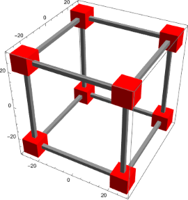
We visualize this results of the optimization solution. The left view is in the world coordinate system: the black arrow represents the center line of view, the thin red line is the 3D cube, the thick red line is its projection on the 2D image plane, and the green line is the projection ray. The right view is a cube projected onto a 2D canvas in the camera coordinate system. Their position and orientation can be compared against the orange sampled points.
Out[]=


3. reconstructing Escher’s cube
3. reconstructing Escher’s cube
3.1 modeling Escher’s 3D cube
3.1 modeling Escher’s 3D cube
3.1.1 creating one-period cube
3.1.1 creating one-period cube
Create a one-period Escher’s cube.
In[]:=
cubidX[x_,y_,z_]:=Cuboid[{-x,y-1,z-1},{x,y+1,z+1}];cubidY[x_,y_,z_]:=Cuboid[{x-1,-y,z-1},{x+1,y,z+1}];cubidZ[x_,y_,z_]:=Cuboid[{x-1,y-1,-z},{x+1,y+1,z}];cubidT[x_,y_,z_,r_]:=Cuboid[{x-r,y-r,z-r},{x+r,y+r,z+r}];
In[]:=
cXYZ=With[{d=1*25,s=50},Table[{cubidX[d,i,j],cubidY[i,d,j],cubidZ[i,j,d]},{i,-d,d,s},{j,-d,d,s}]];cT=With[{d=1*25,s=50},Table[{cubidT[i,j,k,4.5]},{i,-d,d,s},{j,-d,d,s},{k,-d,d,s}]];
In[]:=
Image@Graphics3D[{EdgeForm[None],Gray,cXYZ,Red,cT},Lighting"Neutral",Axes->True,Boxed->True]
Out[]=
In[]:=
objects[{α_,β_,γ_},r_,{x0_,y0_,z0_}]:=GeometricTransformation[{EdgeForm[None],Gray,cXYZ,Red,cT},(TranslationTransform[{x0,y0,z0}].RotationTransform[γ,{1,0,0}].RotationTransform[β,{0,1,0}].RotationTransform[α,{1,0,0}].ScalingTransform[{r,r,r}])];
Using Escher’s view angle, placing Escher’s cube on a 2D image plane.
In[]:=
modelImage=Image@Graphics3D[{{EdgeForm[Purple],Texture[image],Polygon[bounds3D,VertexTextureCoordinates{{0,0},{1,0},{1,1},{0,1}}],Purple,PointSize[0.01],Point[cameraPosition],Point[{-56.55423148932846`,74.38118714288277`,-500}],PointSize[0.01],Green,Point/@bounds3D},{objects[{1.34,0.9,0.76},1,{3.9,105.4,60.1}]}},Boxed->False,ImageSize->500{1,1},ViewVector{cameraPosition,{-56.55423148932846`,75.38118714288277`,-1500}},Background->Lighter@LightGray,ViewAngle65*Degree];
3.1.2 create multi-period cube
3.1.2 create multi-period cube
Create more periods Escher’s cube.
In[]:=
cubidX[x_,y_,z_]:=Cuboid[{-x-50,y-1,z-1},{x+50,y+1,z+1}];cubidY[x_,y_,z_]:=Cuboid[{x-1,-y,z-1},{x+1,y,z+1}];cubidZ[x_,y_,z_]:=Cuboid[{x-1,y-1,-z},{x+1,y+1,z}];cubidT[x_,y_,z_,r_]:=Cuboid[{x-r,y-r,z-r},{x+r,y+r,z+r}];
In[]:=
cXYZ=With[{d=11*25,s=50},Table[{cubidX[d,i,j],cubidY[i,d,j],cubidZ[i,j,d]},{i,-d,d,s},{j,-d,d,s}]];cT=With[{d=11*25,s=50},Table[{cubidT[i,j,k,4.5]},{i,-d,d,s},{j,-d,d,s},{k,-d,d,s}]];
In[]:=
objects[{α_,β_,γ_},r_,{x0_,y0_,z0_},d_]:=GeometricTransformation[{cXYZ,cT},(TranslationTransform[{x0,y0,z0}].RotationTransform[γ,{1,0,0}].RotationTransform[β,{0,1,0}].RotationTransform[α,{1,0,0}].TranslationTransform[{d,0,0}].ScalingTransform[{r,r,r}])];
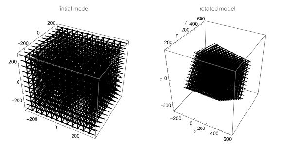
The graphics on the left shows Escher’s multi-period cube, initial model. The graphics on the right shows Escher’s multi-period cube after its rotated.
In[]:=
Image@GraphicsRow[{Graphics3D[{objects[{0,0,0},1,{0,0,0},0]},Axes->True,Boxed->True,Lighting"Accent",ImageSize->300,PlotLabel->"intial model"],Graphics3D[{objects[{1.34,0.9,0.76},1,{3.9,105.4,60.1},200]},Lighting"Accent",Axes->True,Boxed->True,ImageSize->300,AxesLabel{"x","y","z"},PlotLabel->"rotated model"]},ImageSize->600]
Out[]=
3.2 more Escher’s graphics techniques
3.2 more Escher’s graphics techniques
3.2.1 lighting
3.2.1 lighting
In analyzing Escher’s strategy of using light, another of his works gives us a lot of inspiration. In the image, a man’s powerful hands try to climb out of a deep and dark well. At the wellhead position, the upper center of the image, presents a strong white light illumination, creating a strong contrast between light and dark.
In[]:=
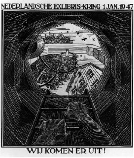
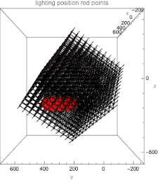
Lighting design:For the cubic spaces described in this article, we have reason to believe that Escher using similar lighting strategies, but more strong light transmittance. Directly on center upwards of the image, it was originally a light opening position of the periodic cube lattice structure, which is a more transparent hole than any other position. By increasing of the number of periods, the lighting position will have a minimal effect, which will not be covered by the edges of the new periodic cube. Escher placed a strong illuminating light source here, then he gradually changes grayscale from light source to the backlight of close structure.
Based on the above analysis, we have arranged a row of horizontal point lights directly in front of the periodic lattice to produce a similar lighting effect, and the position of light source is shown in the red points in the following figure.
In[]:=
Image@Graphics3D[{Lighting{PointLight[Red,{0,-300,0},{0,0,0}]},objects[{1.34,0.9,0.76},1,{3.9,105.4,60.1},200],Red,Opacity[0.7],PointSize[0.1],Point/@Table[{0,200+25*i,-200},{i,8}]},ViewPoint->Left,Lighting"Accent",Axes->True,Boxed->True,ImageSize->300,AxesLabel{"x","y","z"},PlotLabel->"lighting position red points"]
Out[]=
Light-dark boundary enhance:At the same time, Escher uses a “white line edge” in the boundary between space and structure, to further enhance the contrast effect of light and solid. Here we take a simplified approach by directly assigning all cubic edge form to white. It could be simulated using ray tracing or complex algorithms.
Control grayscale of the face: In a traditional lithograph, there are actually only two colors, either black or white. Escher successfully constructed the illumination effect of the light and the perspective effect of the extension of the space by controlling the gray level on the each face of cube in space. A solid backlight facing near viewer is produced, and a discrete gradient transitions to the bright light position in the center, where it is white center of the strong illuminating light. In this area, structure is invisible, period is unpredictable.
3.2.2 texture
3.2.2 texture
In addition, Escher has made stipple shading texture for close-up structural to further perform solid of material. For Stipple Shading, see Silvia’s article, reference [4].
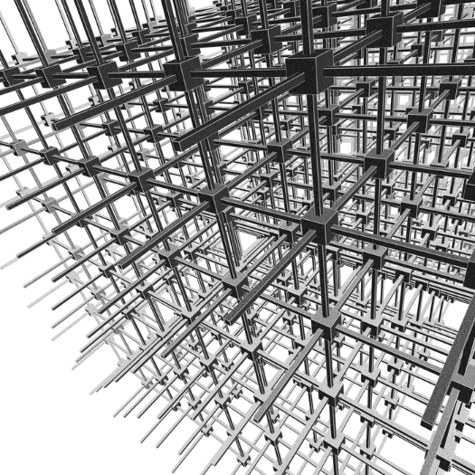
Finally, we integrate all above techniques and processing into the code to reproduce a complete image.
In[]:=
finalImage=Image@Graphics3D[{{LightingJoin[Table[PointLight[GrayLevel[.5],{0,200+25*i,-200},{0,0,1}],{i,8}],{PointLight[GrayLevel[.5],{0,0,300},{0,0,1}]}],EdgeForm[GrayLevel[.9]],FaceForm[Directive[StippleShading[],GrayLevel[.15]]],objects[{1.34,0.9,0.76},1,{3.9,105.4,60.1},4*50]}},PlotRange600{{-1,1},{-1,1},{-1,1}},Lighting"Accent",Boxed->False,ImageSize->1400{1,1},ViewVector{cameraPosition,{-56.55423148932846`,75.38118714288277`,-500}},ViewAngle65*Degree];ImageResize[finalImage,{700,700}]
Out[]=
3.2.3 boundary
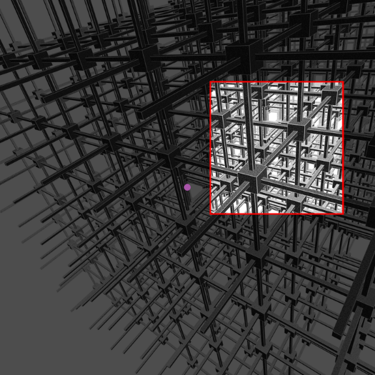
3.2.3 boundary
Use the Escher’s view boundary and hide the rest of the structure. The specific boundary avoids the simple copy and repetition of periodic structures. The structures in the boundary looks all different, actually they are all the same. This psychology conflict impacts and confuses its reader.
In[]:=
imageBoundary={{785,602},{1280,1095}};ImageResize[HighlightImage[finalImage,{Red,Rectangle@@imageBoundary,Lighter@Purple,Point[{700,700}]},"Darken"],{700,700}]
Out[]=
3.3 comparison
3.3 comparison
In[]:=
ColumnRow[Style[#,18,Bold]&/@{" Escher's original work","author's approach"," image difference"},Spacer[65]],GraphicsRowa=ImageResizeImageCrop@
,700{1,1},b=ImageResize[ImageTake[finalImage,{305,800},{785,1285}],700{1,1}],c=ImageDifference[a,b],ImageSize800,Row[ImageHistogram[#,ImageSize->235,Frame->True,ImageMargins->15]&/@{a,b,c}],Alignment->Left;
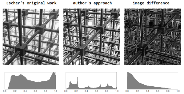
Compare the works: the upper left picture is Escher’s original work, the upper middle image is the author’s approach, and the upper right image shows the pixel difference between the two works. The three sub-plots in the following are the grayscale distribution corresponding to the image in the above figure, respectively.
4. extend Escher’s method
4. extend Escher’s method
4.1 apply Escher’s view techniques
4.1 apply Escher’s view techniques
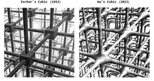
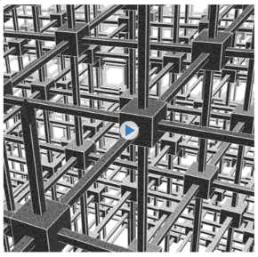
Escher’s legacy and techniques of perspective aesthetics can be used to visualize many complex structure, like triply periodic minimal surface lattice (TPMS). As shown in below, the left image is Escher’s original work. The right image shows that a cubic based lattice structure. The author replaced Escher’s cube model by a triple periodic minimal surface lattice structure, but the view setting are same as Escher’s. This special internal view clearly reveals a complex structure of lattice at first sight.
4.2 animation: Escher’s periodic cubic to Infinite
4.2 animation: Escher’s periodic cubic to Infinite
In Escher’s another works (Depth), the perspective is also that the center line of view located outside the image boundary, and principal point is near the left side of image boundary. The perspective method of Depth is almost same as Cubic Space Division.
Out[]=
Source: M.C. Escher, Depth, wood engraved, 1955.
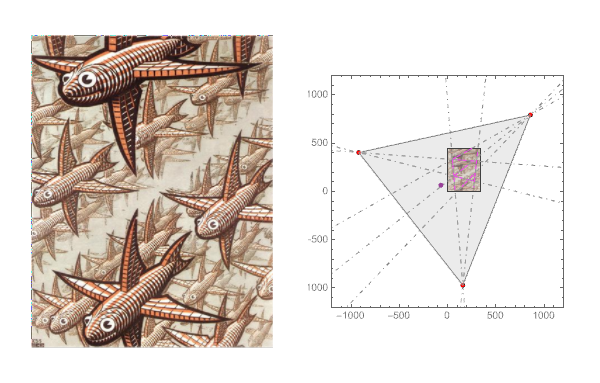
Inspired by Depth, there are many flying fishes. They appear to be dynamically flying forward. If Escher could have a computer and Mathematica in his time, he would probably have wanted to make an animation like the following.
So, we generate an animation to for Escher’s infinite cube flight by moving the lattice one period in the forward direction.
In[]:=
cubidX[x_,y_,z_]:=Cuboid[{-x-50,y-1,z-1},{x+50,y+1,z+1}];cubidY[x_,y_,z_]:=Cuboid[{x-1,-y,z-1},{x+1,y,z+1}];cubidZ[x_,y_,z_]:=Cuboid[{x-1,y-1,-z},{x+1,y+1,z}];cubidT[x_,y_,z_,r_]:=Cuboid[{x-r,y-r,z-r},{x+r,y+r,z+r}];
In[]:=
cXYZ=With[{d=11*25,s=50},Table[{cubidX[d,i,j],cubidY[i,d,j],cubidZ[i,j,d]},{i,-d,d,s},{j,-d,d,s}]];cT=With[{d=11*25,s=50},Table[{cubidT[i,j,k,4.5]},{i,-d,d,s},{j,-d,d,s},{k,-d,d,s}]];
In[]:=
objects[{α_,β_,γ_},r_,{x0_,y0_,z0_},d_]:=GeometricTransformation[{cXYZ,cT},(TranslationTransform[{x0,y0,z0}].RotationTransform[γ,{1,0,0}].RotationTransform[β,{0,1,0}].RotationTransform[α,{1,0,0}].TranslationTransform[{d,0,0}].ScalingTransform[{r,r,r}])];
In[]:=
images=Table[finalImage=Image@Graphics3D[{LightingJoin[Table[PointLight[GrayLevel[.5],{0,200+25*i,-200},{0,0,1}],{i,8}],{PointLight[GrayLevel[.5],{0,0,300},{0,0,1}]}],EdgeForm[GrayLevel[.9]],FaceForm[Directive[StippleShading[],GrayLevel[.15]]],objects[{1.34,0.9,0.76},1,{3.9,105.4,60.1},4*50-i]},PlotRange600{{-1,1},{-1,1},{-1/1.05,1/3.80}},Lighting"Accent",Boxed->False,ImageSize->1400{1,1},ViewAngle65*Degree,ViewVector{{-56.55423148932846`,74.38118714288277`,260},{-56.55423148932846`,75.38118714288277`,-500}}];ImageTake[finalImage,{305,800},{785,1285}],{i,0,50,2}];
In[]:=
(*ImageDifference[First@images,Last@images]*)
In[]:=
animate=AnimatedImage[Drop[images,-1],FrameRate10]
5. summarize and discussion
5. summarize and discussion
comments for Escher’s work
comments for Escher’s work
1
.Minimalism and Complexity: Escher’s work is the contradiction and unity of minimalism and complexity. As one of the simplest 3D solids, the cube transformed into an extremely complex, large spatial structure through a periodic structure in Escher’s hands. In addition, he involved a very special three-point perspective method and image boundary trimming technique, resulting in a visual experience that is intersected and interwoven back and forth, and the continuity is endless.
2
.From one to infinite: The idea of going from one to infinite is reflected in many of Escher’s works, including this one. One that you can say that he painted only one cube or a finite number of cubes, and at the same time it can be said that he painted an infinite number of cubes.
3
.Precise drawing: Escher drew very precisely, and the only tools of his time were mostly rulers and compasses. The vanishing points can be found in a narrow area of intersection points of orthogonal structural line. The maximum angle error for Escher’s lines is about 0.00027 Rad or 0.015 degree.
4
.Linear perspective: The work fully conforms to the principle of linear perspective, in the meantime, it runs out of the frame of the art academy and traditional perspective. There are two differences compared with the traditional three-point perspective: 1. The horizon is not horizontal, and the author conjectured that Escher wanted to use the first horizontal bar to simulate a false horizontal line, and produce the effect of illusion. 2. The center line of view and the principal point are outside the image boundary. If you use traditional three-point perspective to reproduce his image, you will never find that particular perspective image. This kind of perspective technique exist in several Escher’s subsequent works, and they are by no means of unique.
5
.3D periodic cubic lattice structure: Through the reconstruction method described in this article, it can be determined that the geometric model of this work is a periodic cubic lattice structure, which is also consistent with the name of the work. Escher is reputed by his 2D tessellations of periodic patterns. This work can also be regarded as the foundational work of his approach towards a 3D periodic structure, or a basic ideas on the division of spatial networks in 3D.
6
.Lighting, control grayscale : Escher makes full use of the opening hole of the cubic lattice structure at a specific angle of view, which is located directly above the center of the image, and uses lighting to produce a strong illuminating effect, giving the viewer an infinite iteration of structure. Since it is a traditional lithograph, while only two colors, black or white, are available. Escher constructs the illumination effect of the light and the perspective effect of the extension of the space by controlling the grayscale on the end face of each cube. A solid backlight facing near viewer is produced, and a discrete gradient transitions to the bright light position in the center, where it is white center of the strong illuminating light. In this area, structure is invisible, period is unpredictable.
7
.Image boundary: The specific image boundary avoids the simple copy and repetition of periodic structures. The structures in the boundary looks all different, actually they are all the same. This psychology conflict impacts and confuses its viewer.
further improvement
further improvement
1. In this article, the position and orientation of the model are optimized. The distance between the perspective projection of 8 cubic vertices and 8 image sampled vertices are measured. The target optimization function is to minimizing the total distance of 8 vertices pairs to obtain an approximate solution. However, the approximate solutions are not unique, and there are many or even infinite solutions. Alternatively, target optimization functions can be refined, such as minimizing differences of face or minimizing differences for region or area.
2. Escher uses a “white line edge” in the boundary between space and structure, to further enhance the contrast effect of light and solid. Here we take a simplified approach by directly assigning all cubic edge form to white. It could be improved using ray tracing or other complex algorithms.
3. This article does not know exactly the position of lighting source and intensity distribution, so the overall and local grayscale is still quite different from the original. However, according to the grayscale value one each cubic face, light intensity distribution and the lighting source position can be rediscovered someday.
reference
reference
[1] B. Ernst, The Magic Mirror of M. C. Escher, Köln: Taschen Press, 2018. pp.46-49.
[3] I. Hafner, “Perspective Projection of a Cube onto a Plane”, Wolfram Demonstrations Project, 2017.
CITE THIS NOTEBOOK
CITE THIS NOTEBOOK
The perspective of Escher's cubic space division
by Frederick Wu
Wolfram Community, STAFF PICKS, September 4, 2022
https://community.wolfram.com/groups/-/m/t/2611046
by Frederick Wu
Wolfram Community, STAFF PICKS, September 4, 2022
https://community.wolfram.com/groups/-/m/t/2611046