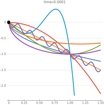
Arbitrary descent trajectory
Arbitrary descent trajectory
The role of the functionINPUT: Expression of orbit----y[x] , e.g.CALCULATE:the Lagrangian, and the left hand side of the Lagrange Equation ,其中 OUTPUT:A second order ordinary differential equations with respect to the Generalized CoordinatesTHE CORE PROBLEM:Solve the Lagrange equation, acquire the expression of x[t].
1-
2
(x-1)
lhs=-
d
dt
∂L
∂
•
q
∂L
∂q
q=x
lagrangianEquation[expr_]:=Module{rule,lagrangian,left,eqn,solx,soly},rule={y[x]->expr,y'[x]->D[expr,x],y''[x]->D[expr,{x,2}]}/.{x->x[t]};(*Transformationrulestobeusedinthelaststep*)lagrangian=m(+)+mgy[x[t]];(*TheLagrangianiscompoundedusingx[t],andtheindependentvariablesinthisequationare:generalizedcoordinatesandgeneralizedvelocity.*)(left=(D[D[lagrangian,x'[t]],t]-D[lagrangian,x[t]])//Simplify);Simplify[(left=left/.rule)==0,Assumptions->{x[t]!=0,x'[t]!=0,x''[t]!=0}]lagrangianEquation[y[x]]//Simplify//TraditionalFormlagrangianEquation[x]lagrangianEquation[2x]lagrangianEquation[
1
2
2
x'[t]
2
(y'[x[t]]x'[t])
x
]Out[]//TraditionalForm=
m(x(t))(t)(x(t))-g+(t)(x(t))+(t)0
′
y
2
′
x
′′
y
′′
x
2
′
y
′′
x
Out[]=
gm2m[t]
′′
x
Out[]=
2gm5m[t]
′′
x
Out[]=
m4g+[t]-2x[t][t]-8[t]0
3/2
x[t]
2
′
x
′′
x
2
x[t]
′′
x
In[]:=
ε=0.0001;tLast=3;Clear[x,y,m,g];tracks=Sqrt[x],x,,Sinx,Sin[10πx],BesselJ[1/2,x];solutionsOfLagrangeEquation=(NDSolve[{lagrangianEquation[#]/.{m->1,g->9.8},x[ε]==ε,x'[ε]==ε},x[t],{t,ε,tLast}][[1]])&/@tracks;Tracks=-tracks;Manipulate[Show[Plot[Tracks,{x,0,1.5},PlotTheme->"Business",PlotLabel->"time="<>ToString[tt],PlotLegends->Evaluate[ToString[#,TraditionalForm]&/@tracks],AspectRatio->1],Graphics[{Black,PointSize[0.03],Point[Evaluate[({x[t],-tracks[[#]]/.x->x[t]}/.solutionsOfLagrangeEquation[[#]])&/@Range[Length[tracks]]]/.t->tt]}]],{tt,ε,tLast},SaveDefinitions->True]
2
x
π
2
1-
,LegendreP[5,x],x+2
(x-1)
1
10
Out[]=


In[]:=
Export["fall.gif",Table[Show[Plot[Tracks,{x,0,1},PlotTheme->"Business",PlotLabel->"time="<>ToString[ttt],PlotLegends->Evaluate[ToString[#,TraditionalForm]&/@tracks],AspectRatio->1],Graphics[{Black,PointSize[0.03],Point[Evaluate[({x[t],-tracks[[#]]/.x->x[t]}/.solutionsOfLagrangeEquation[[#]])&/@Range[Length[tracks]]]/.t->ttt]}]],{ttt,ε,1.5,0.03}],"DisplayDurations"->0.1]
Out[]=
fall.gif
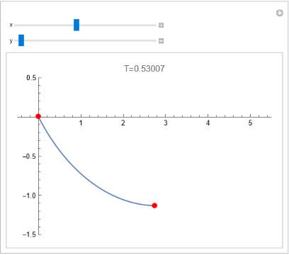
The shortcut line drops
The shortcut line drops
Orbit
Orbit
p
2
∫
p
1
2
′
y
2gy(x(t))
In[]:=
F=;(*Theformoftheequationiscalculated*)Simplify[(D[D[F,y'[x]],x]-D[F,y[x]])==0,Assumptions->{y[x]!=0,y'[x]!=0,g>0}]
1+
2
y'[x]
2gy[x]
Out[]=
1+[x]+2y[x][x]
2
′
y
′′
y
3/2
g1+[x]
2
′
y
y[x]
In[]:=
ε=0.001;curve[X_,Y_]:=Module{sol,point,T,g=9.8},sol=NDSolve[{1+[x]+2y[x][x]==0,y[1]==1,y[X+1]==Y+1},y[x],{x,1,X+1}];point=Table[{x-1,-y[x]+1}/.sol[[1,1]],{x,1,X+1,0.01}];T=NIntegrateEvaluate/.sol[[1,1]]/.{y'[x]->D[y[x]/.sol[[1,1]],x]},{x,1,X+1};ListLinePlot[point,PlotRange->{{-0.5,5.5},{0.5,-1.5}},Epilog->{PointSize[Large],Red,Point[{{0,0},{X,-Y}}]},PlotLabel->"T="<>ToString[T]]Manipulate[curve[x,y],{x,1,5},{y,1,5}]
2
′
y
′′
y
1+
2
y'[x]
2gy[x]
Out[]=
In[]:=
Export["2.jpg",curve[2,1]]
Out[]=
2.jpg
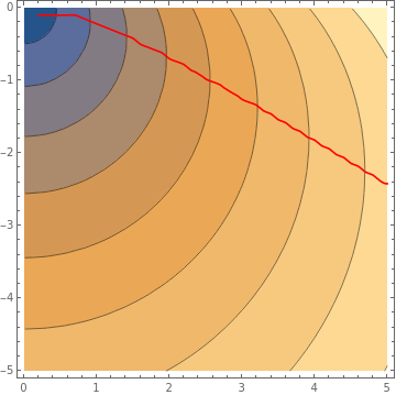
The time of fall
The time of fall
In[]:=
Time[X_,Y_]:=Module[{sol,T,g=9.8,y},sol=NDSolve[{1+Derivative[1][y][x]^2+2y[x](y''[x])==0,y[1]==1,y[X+1]==Y+1},y[x],{x,1,X+1}];T=NIntegrate[Sqrt[(1+y'[x]^2)/(2gy[x])]/.sol[[1,1]]/.{y'[x]->D[y[x]/.sol[[1,1]],x]},{x,1,X+1}]]redPoints=FindMinimum[Time[#,y],{y,1}]&/@Range[0.01,5,0.01]//Quiet;
points={#,MinimalBy[Table[{yy,Time[#,yy]},{yy,0.1,3,0.04}],Last][[1,1]]}&/@Range[0.2,5,0.1];Show[pic,Plot[Interpolation[{#[[1]],-#[[2]]}&/@points,x],{x,0.2,5},PlotStyle->Red]]
Out[]=
CITE THIS NOTEBOOK
CITE THIS NOTEBOOK
Brachistochrone problem: shortest time to slide on a curve
by Yaosheng Zhang
Wolfram Community, STAFF PICKS, March 25, 2023
https://community.wolfram.com/groups/-/m/t/2859015
by Yaosheng Zhang
Wolfram Community, STAFF PICKS, March 25, 2023
https://community.wolfram.com/groups/-/m/t/2859015