ABSTRACT (original article): Microgravity environments present unique movement and perceptual challenges which are most appropriately explored by movement professional. The high cost of microgravity and space endeavors place utilization of the time in those environments at a premium. We have identified techniques which can be practiced on Earth to increase competence of motion and develop a deeper understanding of reorientation of the human body in microgravity. This research has focused on understanding strategies for planning and executing specific movements, which can be explored in precise and low cost ways. A simulator was coded to explore the dynamics of the human body, which allows for visual and numeric calculations of the body’s moment of inertia eigenvectors and center of mass in a variety of positions. The maneuvers were explored with dance, circus, and parkour artists through the use of parabolic flights, pools, and aerial harnesses. CITATION (original article): R. Adam Dipert (2021), Choreographic techniques for human bodies in weightlessness, Acta Astronautica, Acta Astronaut. 182, 46–57. https://doi.org/10.1016/j.actaastro.2021.02.001
Full related videos playlist
Full related videos playlist
But what does juggling in space look like?
When I ask that question, I’m not wanting to just take Earth juggling and put it in space. I wanted to find out what juggling would look like for a space artist. I worked hard to figure out the technique and practice it. A couple of weeks ago, I even won first place in the International Jugglers’ Association 2021 Championship Competition with a Space Juggling performance!
This notebook is part of a much larger work to answer this question about juggling in space. Check out more about the project at www.theSpaceJuggler.com.
Moment of Inertia of Human Body
Moment of Inertia of Human Body
Before my first parabolic flight, I wrote a Mathematica code to calculate the principal moments of inertia of the human body in different positions. The article outlining some of that research is called "Choreographic Techniques for Human Bodies in Weightlessness" The image below was generated using that notebook.

Knowing the principal axes is useful because the maximum and minimum axes show us what axes we can rotate around stably. If the system doesn't have degeneracies, these are the only axes the body can rotate around stably. The axes are found by constructing the moment of inertia tensor (about the center of mass of the body) then finding the eigenvalues and eigenvectors.
In the figure above, the blue and red arrows represent the maximum and minimum axes, respectively. If the body's total angular momentum is aligned with one of these axes, the body will rotate stably and won't wobble. I found it interesting that the body can rotate around the belly, kind of like a cartwheel by spinning around the blue axis.
In the figure above, the blue and red arrows represent the maximum and minimum axes, respectively. If the body's total angular momentum is aligned with one of these axes, the body will rotate stably and won't wobble. I found it interesting that the body can rotate around the belly, kind of like a cartwheel by spinning around the blue axis.
Throwing Balls in Weightlessness
Throwing Balls in Weightlessness
The next detail to understand is that when a ball is thrown in weightlessness, it travels in a straight line rather than a parabola.
We can put these two pieces of information together by considering that a person could spin around in a cartwheel kind of motion and throw balls down to themselves. Even more interestingly, we know the balls travel in straight lines in inertial space but what path do they travel in the rotating frame? What does the juggler see?
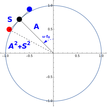
First, we need a function which represents the orientation of the juggler's spine. Let's say the distance from the head to the position along the spine and between the juggler's hands is A. We can also say the juggler is spinning with angular velocity ω. Thus
We can put these two pieces of information together by considering that a person could spin around in a cartwheel kind of motion and throw balls down to themselves. Even more interestingly, we know the balls travel in straight lines in inertial space but what path do they travel in the rotating frame? What does the juggler see?
First, we need a function which represents the orientation of the juggler's spine. Let's say the distance from the head to the position along the spine and between the juggler's hands is A. We can also say the juggler is spinning with angular velocity ω. Thus
In[]:=
f[t_]:=A*Exp[ωt];
We want to know the offset from the point f[t] to the positions of the hands, and we can just scale and rotate f[t] to keep things simple.
In[]:=
g[t_]:=S*f[t];
Remember that multiplying any complex vector by a unit complex number rotates it by the angle between positive real axis and the vector.In Mathematica terms, if you have a unit complex vector, you can calculate the Arg of the vector and it will tell you what the rotation angle is.
If we add f[t] and g[t], we’ll have a location for the left hand.
If we add f[t] and g[t], we’ll have a location for the left hand.
In[]:=
PL[t_]:=f[t]+g[t];
If we subtract g[t] from f[t], we' ll have the location of the right hand.
In[]:=
PR[t_]:=f[t]-g[t];
Let' s just take a quick look at what we' ve got so far. We' ll set ω = 2 π, so that values of t are simply proportional to the number of revolutions. Let's set so we can see it off an axis.
t=1/8
In[]:=
A=1;S=0.3;ω=2π;t=1/8;ShowFullCircle=ParametricPlot[{Sin[t],Cos[t]},{t,0,2π},ImageSizeMedium],GraphicsPointSize[0.05],Black,Point[{ReIm[f[t]]}],Red,Point[{ReIm[PL[t]]}],(*LeftHandLocation*)Blue,Point[{ReIm[PR[t]]}],(*RightHandLocation*){Black,Line[{ReIm[PL[t]],ReIm[PR[t]]}],(*lineconnectinghands*)Line[{ReIm[f[t]],{0,0}}],(*linefromcenteralongspine*)Dashed,Line[{ReIm[PL[t]],{0,0}}]},(*arc*){Dashed,Opacity[1.0],Arrow[BSplineCurve[Table[0.3*{Cos[x],Sin[x]},{x,π/2,π/2+ωt,Pi/20}]]]},(*Text*)Text[Style["S",Large,Bold],ReIm[f[t]-0.2]],Text[Style["A",Large,Bold],ReIm[f[t]*0.5+0.2]],TextStyle"+",Large,Bold,ReIm[f[t]*0.5-0.2-0.35],Text[Style["ω ",Medium,Bold],{-0.15,0.35}]
2
A
2
S
t
0
Out[]=
Now we've got a way to represent how the body is going to rotate in the cartwheel motion. The next we need a representation of a ball moving.It's going to move in a straight line. We want it to start in one of the juggler' s hands and we want it to be caught in one of the juggler's hand. Mathematically, that means the trajectory will begin at time in position []=PL[] or []=PR[] and it will end at a time τ later in position [+τ]=PL[+τ] or [+τ]=PR[+τ].The vector representing the direction the ball is traveling is The location of the ball in space starts at the initial point, then travels during a time τ, therefore the trajectory of the line in inertial space isWe can plot these trajectories. See the line on the left plot below.
t
i
P
i
t
i
t
i
P
i
t
i
t
i
P
f
t
i
t
i
P
f
t
i
t
i
B[,τ]=[+τ]-[]
t
i
P
f
t
0
P
i
t
0
TL[,τ]=B[,τ]+[]
t
0
t-
t
0
τ
t
0
P
i
t
0
In[]:=
ManipulateAnimateA=1;scale=0.2;f[t_]:=A*Exp[ωt];g[t_]:=scale*f[t];(*Plotcirclestomakeanimationsteadyandsimple*)FullCircle=ParametricPlot[{Sin[t],Cos[t]},{t,0,2π},ImageSize290];FullCircle2=ParametricPlot[{Abs[f[0]+g[0]]*ReIm[f[t]]},{t,0,4},ImageSize290,PlotStyleDashed];PL[t_]:=f[t]+g[t];PR[t_]:=f[t]-g[t];TL[T_,τ_]:=(p2[τ]-p1[0])*(T/τ)+p1[0];Row(* +++++++++FIRSTCOLUMN+++++++++*)Show[{FullCircle,FullCircle2,Graphics[{Text["τ = "+τ,{-0.85,0.95}]}],(*Hands-LeftandRightLines-TorsoandShoulders*)Graphics[{PointSize[0.05],Black,Point[{ReIm[f[T]]}],Red,Point[{ReIm[PL[T]]}],(*LeftHand*)Blue,Point[{ReIm[PR[T]]}],(*RightHand*)Black,Line[{ReIm[PL[T]],ReIm[PR[T]]}],Black,Line[{ReIm[f[T]],{0,0}}]}],Graphics[{PointSize[0.05],(*Ball1*)(*startpoint*)Green,Point[{ReIm[p1[0]]}],(*endpoint*)Point[{ReIm[p2[τ]]}],(*BallTrajectoryinWorldSpace*)Point[{ReIm[TL[T,τ]]}],{Black,Text[Style["Non Rotating Frame",18,Bold],{0,-0.5},BackgroundWhite]}}],(*Ball1*)(*Plotlineconnectingp1andp2*)ParametricPlot[ReIm[TL[Τ,τ]],{Τ,0,τ}],(*plotrotatingtrajectoryininertialframe--dotted*)(*TRLvariableiscontrolledinMantipulateoptions,itturnstheploton/off*)ParametricPlot[TRL*ReIm[-f[T]*f[-Τ]*TL[Τ,τ]],{Τ,0,τ},PlotStyleDashed]}],(* +++++++++SECONDCOLUMN+++++++++*)Show[{FullCircle,FullCircle2,(*plotrotatedtrajectory*)ParametricPlot[ReIm[-f[-Τ]*TL[Τ,τ]],{Τ,0,τ}],Graphics[{PointSize[0.05],(*GeneratesrotatedpointB1*){Purple,Point[{ReIm[-f[-T]*TL[T,τ]]}]},Text[Style["Rotating Frame",18,Bold],{0,-0.5},BackgroundWhite]}]}],(*Animateparameters*){T,0,τ},AnimationRate0.05,AnimationRunningFalse,(*Manipulateparameters*){{p1,PR,"Ball 1 throw"},{PR,PL}},{{p2,PL,"Ball 1 catch"},{PR,PL}},{{TRL,0,"Show rotated trajectory in inertial frame"},{0,1}},{{ω,-6.28319,"Rotational Velocity ω (intial value is -2π)"},Table[nπ,{n,-2,2,0.5}]},{{τ,0.4,"Full Rotations To Catch τ"},0.1,2},SaveDefinitionsTrue
Out[]=


What's even more interesting is seeing the trajectories in the rotating frame. The right figure above shows what the juggler sees in the rotating frame. Do you notice how the balls are moving in arcs?
To generate the plots in the rotating frame, as seen on the right above, you just need to multiply the line function TL by an exponential rotating in the opposite direction at the same angular velocity.
To generate the plots in the rotating frame, as seen on the right above, you just need to multiply the line function TL by an exponential rotating in the opposite direction at the same angular velocity.
Archimedean Spirals
Archimedean Spirals
Let’s take a closer look at the equation which represents the ball throws. To simplify we can consider that we don’t really need the imaginary term outside the exponential because it just represents a rotation. And we can define g[t] in a more convenient way. Hang with me on the next set of equations. By the end of this section, you will see why I chose to take us down this path.f[t] = A Exp[ ω t ]g[t] = S Exp[ ω t ]giving a different version of the equations for the locations of the left PL and right PR hands as functions of timePL[t] = A Exp[ ω t ] + S Exp[ ω t ]PR[t] = A Exp[ ω t ] - S Exp[ ω t ]which we could rewrite asPL[t] = ( A + S ) Exp[ ω t ]PR[t] = ( A - S ) Exp[ ω t ]for convenience, we could define=ASWhere + is used for the left hand location and - is used for the right hand location. We can now compress these into a single statement Adopting one more convention, we can represent the throw as i or catch as f. Giving us the positions of the throw and catch as Pi[i] and Pf[t], respectively.The direction the ball travels is We can now rewrite the equation for the linear trajectory of a ball. Recall that the throw will happen at time and the catch will happen a time τ later.Now to rotate our view of the ball trajectories, we rotate this entire system in the opposite direction by multiplying by .This is actually the same function as we plotted above in the rotating frame. However, if we take a look at where our time variable ended up, we can see that the equation just has an exponential terms times a linear term. We could set =0, and write and . Now the equation takes the formThat’s the equation for an Archimedean Spiral.Of course, this equation usually only has a,b ∈ while in our equation we allow a,b ∈ .
Ω
k
±
k
Pk[t]=Exp[ωt]
Ω
k
B[t,τ,ω]=Pf[t+τ]-Pi[t]=-=(-)
Ω
f
ω(t+τ)
e
Ω
i
ωt
e
ωt
e
ωτ
e
Ω
f
Ω
i
t
0
TL[t,τ,ω]=B[t,τ,ω]+Pi[t]=(-)+=(-)+
t-
τ
0
τ
t-
τ
0
τ
ωt
e
ωτ
e
Ω
f
Ω
i
Ω
i
ωt
e
ωt
e
t-
τ
0
τ
ωτ
e
Ω
f
Ω
i
Ω
i
Exp[ωt]
T=*TL[,ω,τ]=(-)+=(-)+
-ωt
e
t
0
-ωt
e
ω
t
0
e
t-
τ
0
τ
ωτ
e
Ω
2
Ω
1
Ω
1
-ω(t-)
t
0
e
t-
τ
0
τ
ωτ
e
Ω
2
Ω
1
Ω
1
t
0
a=(-)
1
τ
ωτ
e
Ω
2
Ω
1
b=
Ω
1
T=(at+b)
-ωt
e
Coriolis and Centrifugal Forces
Coriolis and Centrifugal Forces
The Coriolis force is often thought of within the context of the entire Earth spinning. I.e. hurricanes or water draining. When written using linear algebra, the force is expressed as =-2m(ωxv'), where m is the mass of the object, ω is the angular velocity and v’ is the velocity of the object in the rotating frame.The centrifugal force is usually thought of in the terms of cars turning quickly or being inside of a spinning carnival ride. Using linear algebra, we would write the force as =-mωx(ωxr'), where r’ is the position of the object in the rotating frame.These forces are interesting because they are the most common forms of “fictitious forces”, a term which often is very confusing. My confusion often stemmed from the fact that we use physical systems with actual forces acting. Like in the case of the hurricanes, there are sections of the air which are further from the axis of rotation (near the equator) and sections of air which are closer (north or south of the equator). That doesn’t seem “fictitious” to me.In the mathematics above, where we’ve thrown a ball along a straight line, we know it is not experiencing any forces, it’s momentum is conserved. However, when we view it in the rotating frame, it follows the Archimedean Spiral. If we check our solution T, we’ll find that T satisfies the differential force equation that includes the Coriolis and centrifugal forces.m a’ = - 2 m (ω x v’) - m ω x ( ω x r’ )We have to either move our complex algebra into linear algebra or vice versa. Let’s find a representation of the differential equation above in complex algebra. First, we write r’ = Tv’ = Ta’ = TNote that the Archimedean spiral is in a plane and that the angular velocity we’ve chosen is perpendicular to that plane. Here’s a quick picture of that system
F
C
F
cent
d
dt
2
d
2
dt
In[]:=
p0={0,0,0};p1={1,0,0};p2={0,1,0};Omega={0,0,1};f[t_]:=Exp[(2π)t]t;Show[{ParametricPlot3D[{ReIm[f[t]][[1]],ReIm[f[t]][[2]],0},{t,-1.5,1.5},BoxedFalse],Graphics3D[{Arrow[{p0,Omega}],(*ωvector*){Blue,Arrow[{p0,p1}],(*RealAxis*)Arrow[{p0,p2}],(*ImaginaryAxis*)},{Opacity[0.4],InfinitePlane[{p0,p1,p2}]},Text[Style["ω",Medium,Bold],1.1*Omega],Text[Style["Re",Medium,Bold],1.15*p1],Text[Style["Im",Medium,Bold],1.15*p2]}]}]
Out[]=

This means that a cross product between ω and any point T, velocity T, or acceleration T on the Archimedean spiral is still in the Real-Imaginary plane. Since it’s a cross product the result is always perpendicular to both input vectors. Thus we can convert the cross product into complex notation by ω x n → ω nwhere n ∈ .We can rewrite our differential equation asT=-2(ω)T-(ω)(ω)TIt’s now time to do the math and see if our solution T satisfies this equation. First let’s take the derivatives, so we can see them.
d
dt
2
d
2
dt
2
d
2
dt
d
dt
In[]:=
T[t_]:=Exp[-ωt](at+b)D[T[t],t]
Out[]=
a-(b+at)ω
-tω
-tω
Simplify the second order derivative
In[]:=
D[T[t],{t,2}];Simplify[%]
Out[]=
-ω(bω+a(2+tω))
-tω
Check the right side of our differential equation
In[]:=
-2(ω)D[T[t],t]-(ω)(ω)T[t];Simplify[%]
Out[]=
-ω(bω+a(2+tω))
-tω
And we can see that each side of the equation is equal to the other
In[]:=
FullSimplify[D[T[t],{t,2}]==-2(ω)D[T[t],t]-(ω)(ω)T[t]]
Out[]=
True
Therefore, we see that this generalized Archimedean spiral trajectory can be described by the Coriolis and centrifugal forces. It this, the fact that these forces are fictitious is quite evident.
Wrap Up
Wrap Up
There is a lot more to explore and understand within the equation T that we found here. For example, go back to the “Rotating and Non-rotating” manipulate object above, run the line again, and put in τ = 0.3. You’ll find a quite interesting result in the rotating frame. Or we could add multiple balls, as is common with juggling, to see how their motions are related to each other in real time.
An interesting discovery that I made during this investigation was that these are the same pathways that all thrown objects will follow in rotating spacecraft. This would apply for everything from the spinning ship on its way to Jupiter in 2001: A Space Odyssey to the rotating Ceres station in The Expanse. Though the rotation rates and radii differences in each of those cases would result in different parts of the spirals shown above to be revealed, the basic trajectories would fit the T function we have found.
I’ve been exploring these equations quite deeply both in Mathematica and in real life using my body. I have developed the Space Juggling technique and you can learn more about it by checking out my website www.theSpaceJuggler.com or on social media Instagram, Facebook, or Twitter (@theSpaceJuggler).
CITE THIS NOTEBOOK
CITE THIS NOTEBOOK
Juggling in space using Archimedean spirals and complex algebra
by R. Adam Dipert
Wolfram Community, STAFF PICKS, July 31, 2021
https://community.wolfram.com/groups/-/m/t/2331903
by R. Adam Dipert
Wolfram Community, STAFF PICKS, July 31, 2021
https://community.wolfram.com/groups/-/m/t/2331903