ABSTRACT (original article): This paper shows a cut along a crease on an origami sheet makes simple modeling of popular traditional basic folds such as a squash fold in computational origami. The cut operation can be applied to other classical folds and significantly simplify their modeling and subsequent implementation in the context of computational origami. CITATION (original article): Tetsuo Ida, Hidekazu Takahashi, A New Modeling of Classical Folds in Computational Origami, Proceedings of the 13 th International Conference on Automated Deduction in Geometry. 352: 41-53. https://doi.org/10.48550/arXiv.2201.00536
We present an application of Eos-implementation of classical origami “flying crane.” Eos (E-origami system) extensively uses Mathematica’s powerful symbolic, algebraic, and graphics capabilities. We employ a new modeling of origami described in the article \cite{ida:2021}. By introducing operations of virtually cutting and gluing the edges of origami faces, we can clarify the notion of fold practised in classical origami. We provide functions that simulate classical folds. Those functions are implemented entirely in Mathematica. We construct a flying crane by programming in Eos programming language Orikoto embedded to the Wolfram Language
1. Introduction
1. Introduction
This post shows an application of the idea that we presented in the paper titled “A New Modelling of Classical Folds in Computational Origami”\cite{2021:ida}. We observe that an origami artwork is a complicated arrangement of bounded two-sided flat planes called faces. They are connected and superposed sophisticatedly by repeated folds of a single shheet of paper. The collection of the faces becomes a remarkable object at the end of construction. We showed in the article that cutting an edge shared by two faces enables a class of classical folds. To glue the faces divided by the cut, we restore the connection of the separated faces. Application of the cut and glue opens the possibility of discovering new folds that are impossible by Huzita-Justin folds~\cite{Huzita: 1989} and~\cite{Justin: 1986}.
The inside-reverse fold is one of the simplest examples of the classical folds but is not in the set of Huzita-Justin folds. Many interesting classical folds are realized by the Huzita-Justin folds plus the cut-and glue operations.
This article shows a further development of the Orikoto programming language based on the new modeling and the construction of a flying crane.
2. Computational Modeling
2. Computational Modeling
Origami is a term meaning “folding paper.” It also refers to a sheet of paper used for origami. Folding an origami along a fold-line and unfolding the folded one to the previous shape leaves a line segment on the origami. It is a part of the fold-line and is called a crease.When we freely choose fold-lines and allow overlaps of faces without breaking the original sheet, we will be able to construct a variety of interesting geometrical objects. On the other hand, when we impose rules of fold-line construction that are mathematically plausible, we can also define an origami geometry that deserves deep mathematical investigation. The Greeks defined Euclidean geometry around 400 B.C. with that spirit. They only used a straightedge and a compass as a tool for constructing geometrical objects. The origami geometry does not use tools but only introduce rules of folding. Huzita-Justin's rules are such rules. Below we list some of Huzita-Justine rules as implemented in Orikoto (3 out of 7 rules) that we use in this post.
For further details, see the monograph "An introduction to computational geometry" \cite{ida:2020}Now coming back to the issue of folding rules, we use Huzita-Justin rules , cut, glue, create arbitrary points on the face, and some more commands by which we rotate faces. We will explain as we go along.
Operation | Huzita-JustinruleinOrikoto |
FoldalongPQ | HO[PQ] |
FoldtobringPtoQ | HO[P,Q] |
FoldtobringPQtoRS | HO[PQ,RS] |
Wedenotetheorigamiatstepiby.
O
i
To run all the programs in this notebook, we need Mathematica 13, the Eos package, and the ClassicalFold package. The latter two will soon be available from the Eos project webpage https://www.i-eos.org. Alternatively, we can enjoy the flying cranes in 3D graphics using Wolfram Player (Wolfram Inc.’s product that we get free of charge).
3. Classical Folds
3. Classical Folds
Mountain fold and Valley fold
Mountain fold and Valley fold
The most elementary fold operations are mountain fold and valley fold. They are called so because the crease looks figuratively like the mountain ridge and valley path. The crease is made by the unfold operation that follows the mountain (or valley) fold. To see how we perform those elementary folds, we try to write a tiny Orikoto program and run it.
Let us suppose at the outset a piece of e-origami colored blue on the front and green at the back. First, we perform a valley fold on the flat origami along the directed line CA, i.e., half-line starting from point A and passing through point C, as shown below (the leftmost one).
In[]:=
EosSession["elementary folds"];
Out[]=
 |  |  |
The result of the valley fold is shown in Fig.1(b). The origami is now two- layered, but the back layer is not visible since the top triangle face completely overlaps the back triangle face. Next, we unfold the origami shown in Fig. 1(c). Unfold does not mean “undoing,” although we recover the shape of the origami to the one in Fig.1(a) except for the dotted line segment CA. We call the line segment valley crease. The line segment looks like a path in the valley if we have a good imagination. In our e-origami, we simulate the situation by looking at the origami lying on the plane precisely from the top right angle. To see the configuration in a way that models the physical space and the origami, we switch to the three-dimensional view mode.
Out[]=
 |  |  |
We construct the origami in Fig.2 (c) by executing the command FO[-0.95 π] [“AC”] instead of Unfold. By this command, we rotate the face ACD by angle of -0.95 π along the half-line AC. we use the right-handed system and select the face to the right of the rotation axis. Rotating an object by angle θ is equivalent to rotating it in a right-hand screw manner. In this case, FO[- π] [“AC”]is operationally Unfold[ ] since the fold-line used by the previous fold (one in Fig.2 (b)) is CA.
Similarly, we have a mountain fold below.
Out[]=
 |  |  |
We noticed that line segment AC is dot-dashed, which represents a mountain crease.
Valley Fold and mountain Fold are also called Inside fold and outside fold, respectively. These names are sometimes more intuitive and help understand the insideReverse fold and outsideReverse fold, which we discuss shortly.
FO
FO
FO, standing for Fold Origami, is a command FO[θ] [faces,ray] for rotating target faces along ray by angle θ. It is a generalization of mountain and valley folds. Note that FO is defined as a Curried function. Using FO, we could define short commands VFold for ValleyFold and MFold for MountainFold. We define them as follows:
In[]:=
VFold=FO[-π];MFold=FO[π];
If faces are omitted, Eos infers the target faces. With θ other than ± π, command FO constructs a 3D origami in general. In such cases, we need careful use of FO. Usually, we use FO[ θ ] at the end steps of the construction.
Inside-reverse and outside-reverse Folds
Inside-reverse and outside-reverse Folds
The inside-reverse and outside-reverse folds are often used methods of folds. Both work on a pair of superposed faces that share an edge. They are combinations of an inside fold and an outside fold. However, each uses inside and outside folds oppositely. In the case of performing the inside-reverse fold by hand, we push the shared edge between the faces and make a valley-like shape. On the other hand, in the case of the outside-reverse fold, we make a triangle cover on the faces. We show simple examples of both folds below.
Inside reverse fold
Inside reverse fold
In[]:=
$markPointOn
Out[]=
{True}
EosSession["Inside-reverse fold"];
In[]:=
NewOrigami[10];
Steps 1 ~ 4 are preparatory. We want two overlapping faces that shared an edge.
In[]:=
VFold["CA"]
Inside reverse fold: Step 2
Out[]=

In[]:=
NewPoint[{"E"{5,5},"F"{10,7}}]
Inside reverse fold: Step 2
Out[]=

In[]:=
HO["FE"]!
Inside reverse fold: Step 4
Out[]=

We have constructed the desired faces. Origami has four faces; faces 6 and 4 are superposing, and so are faces 7 and 5. Moreover, faces 6 and 4 share edge CE.
O
4
To examine the configuration of faces, we provide a special visualization command ShowLayeredFace. It works as follows.
In[]:=
ShowLayeredFace[]
1: {6,7}
During evaluation of In[]:=

2: {4,5}
During evaluation of In[]:=

We should note that the faces form a stack of layers. We slice the collection of faces, and show each slice from top (level 1) to bottom. We push edge EC and insert faces 6 and 4 in between faces 7 and 5. Our next task is to make the superpositions precise.
We see that there are two levels of the stack of faces. The top-level slice consists of two faces, i.e., ΔCEF and polygon ADFE. The numbers placed in the center of the polygons identify the faces and are called face id. The second level, i.e., the bottom level layer, consists of two polygons (one is a triangle). Each is identified by face id 5 or 4. In geometry, vertices are often represented by the point’s name by identifying the edge and the point. It would be too inconvenient to name the faces by the sequence of point names. Eos generates unique numerals to denote the faces, and we use those numerals, i.e., face Ids, in the Orikoto language.
Now we are ready to invoke InsideReverseFold command with list of faces and the fold line as its arguments.
In[]:=
InsideReverseFold[{4,6},"FE"]
Inside reverse fold: Step 8
Out[]=

The command performs two folds; one mountain fold along line EF and the other valley fold along EG. However, this would be impossible, if we simulate “fold by hand,” since edge EC is shared by faces 4 and 6. To do the two folds, we need to cut the faces 4 and 6 along edge EC. Since we are practicing e-origami, we will cut EC. When we finish the two folds. We glue the moved) edge and, we are done. The InsideReverseFold command performs this sequence of operations at one stroke. To examine the result of the operation, we use ShowLayers command.
In[]:=
ShowLayers[Gap1,HingeTrue]
Inside reverse fold: Step 8
Out[]=

We can rotate the Graphics and see the the inside of the stack of layers .
Outside-reverse fold
Outside-reverse fold
An outside-reverse fold is similar to the inside-reverse fold. The only difference is that the outside-reverse fold applies mountain and valley folds to different sides of face layers. Below, we show an example of the use of OutsideReverseFold command in a verbose mode. In this mode, the output of each sub-steps of the command execution are displayed.
In[]:=
EosSession["Outside-reverse fold"];
In[]:=
NewOrigami[10];VFold["CA"];NewPoint[{"E"{7,7},"F"{10,3}}];HO["FE"]!
Outside-reverse fold: Step 4
Out[]=

In[]:=
Block[{$probeFold=True},OutsideReverseFold[{4,6},"FE"]]
CutEdges[{{4,6}}]

MountainFold[4,FE]

ValleyFold[6,FE]

GlueEdges[$cutEdges]
Outside-reverse fold: Step 8
Out[]=

In[]:=
ShowLayers[HingeTrue,Gap0.5,Frame->False]
Outside-reverse fold: Step 8
Out[]=

In[]:=
EndSession[];
Squash fold
Squash fold
Examples best describe squash fold. Orikoto provides four kinds of squash fold commands:
1. Squash rightwards to make a square.
2. Squash leftwards to make a square.
3. Squash rightwards to make a triangle.
4. Squash leftwards to make a triangle.
We show (1) and (2 ) as we will use them to construct a flying crane.
1. Squash rightwards to make a square.
2. Squash leftwards to make a square.
3. Squash rightwards to make a triangle.
4. Squash leftwards to make a triangle.
We show (1) and (2 ) as we will use them to construct a flying crane.
In the session below, Steps 1 - 5 are preparatory to construct the four layers. Each layer has a shape of a right triangle, which consists of (smaller) right triangles.
Squash fold rightwards
Squash fold rightwards
Let us start with the origami at step 5.
In[]:=
EosSession["Squash fold rightwards to square"];
NewOrigami[];HO["A","C"];HO["D","B",Mark{"DB","E"}];HO["C","D"]!
Squash fold rightwards to square: Step 5
Out[]=

Origami is four-layered, and the top layer consists of faces whose Ids are 11 and 10, as we see below.
O
5
In[]:=
ShowOrigami[ShowFaceIdTop,Gap0.1]
Squash fold rightwards to square: Step 5
Out[]=

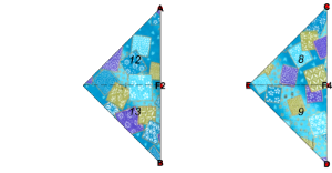
Now, we slide the face 10 rightwards (looking leftwards from the right edge CD) onto face 11 such that segment DE moves onto segment BE. This fold is realized by command SquashFold. We define SquashFold as a Curried function that is to be applied to direction (“L” or “R”), shape (“Square” or “Triangle”), a face list and an an edge list. In this example, {11,10} and {“EC”,”DE”}, respectively. Drawing an analogy of mountain and valley folds, we consider segment DE a ridge and the segment EC as a bottom path. Both segments run on the newly constructed square. Taking those parameters in a structures manner, the SquashFold command here is
SquashFold[“R”][“Square”][{11,10},{“EC”,”DE”}]
When we call the command in the verbose mode, we can see the sub-steps of the command execution. The result of the squash fold is below the message of "Step 10 . " The graphics outputs are displayed in 2D view mode. To see the inner structure of the face layers, we use commnds ShowLayers and ShowLayeredFace.
In[]:=
Block[{$probeFold=True},SquashFold["R"]["Square"][{11,10},{"EC","DE"}]]
CutEdges[{{11,10}}]

ValleyFold[11,Ray[E,C]]

ValleyFold[10,Ray[D,E]]

HO[D,C]

GlueEdges[$cutEdges]
Squash fold rightwards to square: Step 10
Out[]=

In[]:=
ShowLayers[HingeTrue,Gap0.2,ShowFaceIdTop,Frame->False,ImageSize->200]
Squash fold rightwards to square: Step 10
Out[]=

In[]:=
ShowLayeredFace[]
1: {10,14}
During evaluation of In[]:=

2: {15}
During evaluation of In[]:=

3: {12,13}
During evaluation of In[]:=

4: {8,9,11}
During evaluation of In[]:=

In[]:=
EndSession[];
Squash fold leftwards
Squash fold leftwards
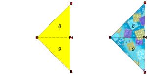
We give SquashFold["L"]["Square"] without further explanation, as we can infer the parameters easily.
In[]:=
EosSession["Squash fold leftwards to square"];
In[]:=
NewOrigami[];HO["D","B"];HO["A","C",Mark{"AC","E"}];HO["A","B"]!;Block[{$displacement=0},ShowOrigami[ShowFaceIdTop,Gap0.1]]
Squash fold leftwards to square: Step 5
Out[]=

In[]:=
Block[{$probeFold=True},SquashFold["L"]["Square"][{10,11},{"EA","BE"}]]
CutEdges[{{10,11}}]

ValleyFold[10,Ray[B,E]]

ValleyFold[11,Ray[E,A]]

HO[A,B]

GlueEdges[$cutEdges]
Squash fold leftwards to square: Step 10
Out[]=

In[]:=
ShowLayers[HingeTrue,Gap0.2,ShowFaceIdTop,Frame->False,ImageSize->200]
Squash fold leftwards to square: Step 10
Out[]=

In[]:=
EndSession[];
4. Flying crane
4. Flying crane
A flying crane origami is an exciting example. It is one of the most popular artworks, and it requires the classical folds that we discussed. Making a fine flying crane by hand is a challenge for beginner origami hobbyists. It involves a considerable degree of skill and gives us a sense of accomplishment when we complete the construction. In the context of computational origami, this example poses yet another challenge in modeling a new class of folds.
In the following, we give the entire steps of constructing a flying crane in Orikoto. Some program codes are added in the description to help us view the internal origami structure.
In this example, we specify the origami surfaces as yellow and textured patterns to make the origami more artistic. A short program code to specify the colors and patterns is not included here,however.
Start of construction
Start of construction
In[]:=
EosSession["Flying crane"];
In[]:=
NewOrigami[16]
Flying crane: Step 1
Out[]=

The essential steps in constructing the crane are to make two overlapping rhombuses. We make them using the petal folds. The rhombuses stretch from NW to SE of the original sheet of paper. Many constructed shapes are symmetric along the diagonal line from NW to SE of the rhombuses. We will have pairs of similar operations; one operates on the left of the diagonal line and the other on the left.
Petal fold
Petal fold
Preparation for a petal fold
Preparation for a petal fold
We first valley-fold along the line DB.
O
1
In[]:=
VFold["DB"]
Flying crane: Step 2
Out[]=

We bring point D to point B by valley-fold . We mark with E the intersection of segment DB and the fold-line.
O
2
In[]:=
HO["D","B",Mark->{{"DB","E"}}]
Flying crane: Step 3
Out[]=

We then fold to bring point B to point C. Note thatpoint B of is shadowed by point D. We mark the intersections of the fold-line and segment BC (and the other three overlapping segments). Let be the resulting origami. By postfix operator !, we unfold and obtain .
O
3
O
3
O
4
O
4
O
5
In[]:=
HO["B","C",Mark->{{"DC","F4","F3","F2","F1"}}]!
Flying crane: Step 5
Out[]=

Origami
O
5
The execution of the following command ShowLayeredFace gives the list of the face Ids on each layer. It displays the layer of faces, and the current origami, i.e., , together with face Ids of its bottom layer, for all levels of . This command is indispensable for us to view the faces on all levels with their Ids. The second graphics view of the origami helps us identify the faces shown in the first graphics view in the entire origami structure. By manipulating the planes of the base-view graphics, we can see the stack of the layers of the faces.
O
5
O
5
In[]:=
ShowLayeredFace[BaseView->True]
1: {10,11}

2: {14,15}

3: {12,13}
4: {8,9}
We are about to apply a squash fold to make a square on the upper half of the right triangle. We have already seem this situation in the subsection of Squash fold rightwards to square.
Squash fold rightwards on the front side
Squash fold rightwards on the front side
In[]:=
SquashFold["R"]["Square"][{10,11},{"EC","DE"}]
Flying crane: Step 10
Out[]=

Point F4 has moved to the above-left corner, and F3 appears at the position where F4 was.
The following command, TurnOver[1], rotates origami across line F3E (Orikoto parses F3E as Segment[F3,G]) by π degree. The argument “1” specifies that the command should turn the whole origami over the initial origami’s central horizontal line. The purpose of executing TurnOver[1] here is to apply the subsequent fold commands to the backside of origami .
O
10
O
10
In[]:=
TurnOver[1]
Flying crane: Step 11
Out[]=

Next, we apply Squash Fold to make a four-layered square to prepare for a petal fold. We check the top layer face Ids of origami .
O
11
In[]:=
ShowLayeredFace[Level->{1}]
1: {8,9,10}

Squash fold leftwards on the back side
Squash fold leftwards on the back side
The following squash fold moves the target faces leftwards and then make the squashed part a square.
In[]:=
SquashFold["L"]["Square"][{8,9},{"EB","CE"}]
Flying crane: Step 16
Out[]=

We now have four-layered square.
Preparation for constructing legs
Preparation for constructing legs
We are in the second phase of the petal construction. We bisect the ∠ EBF2 to make one side of a petal. We superpose the two lines to bisect an angle formed by them. One of Huzita-Justin’s rules can do this. The following command tries to superpose the lines extending segments F2B and EB.
In[]:=
HO["F2B","EB"]
Flying crane: Step 16
Out[]=
 ,
,
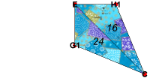
The result would be surprising since we are asked to choose one of the two possibilities. However, it is natural since there are two angle-bisectors. In this case, we want to use the second one and execute the following command, with additional named arguments to mark, with G1, the intersection of the fold-line and the segment F2E. Then, we unfold origami and obtain the following. We notice the valley crease BG1.
O
17
In[]:=
HO[FoldLine->2,Mark->{{"F2E","G1"}}]!
Flying crane: Step 18
Out[]=

Similarly, we obtain the crease BH1.
In[]:=
HO["F1B","EB",FoldLine->2,Mark->{{"F1E","H1"}}]!
Flying crane: Step 20
Out[]=

Left leg by inside reverse fold
Left leg by inside reverse fold
The next step is to make half of the petal, i.e., BG1H1, on the front side. We want to apply InsideReverseFold since we want to use the backside of triangle BG1H1 as the other half of the petal. To apply InsideReverseFold, we need the target face Ids. For this purpose, we execute the command ShowLayeredFace[ and find that face Ids 25 and 27 are the required arguments of InsideReverseFold. We fold along ray BG1.
origami
O
20
Expand the following cell to see the output.
In[]:=
ShowLayeredFace[]
In[]:=
InsideReverseFold[{25,27},"BG1"]
Flying crane: Step 24
Out[]=

Similarly, we prepare the arguments of a face-Id list {17,19} and ray H1B, to make the left part of △ BG1H1.
In[]:=
InsideReverseFold[{17,19},"H1B"]
Flying crane: Step 28
Out[]=

When we rotate the faces 18 and 26 by -π degree along ray H1G1, the petal shape appears on the front side. Note that the fold is a valley-fold along H1G1.
In[]:=
VFold[{18,26},"H1G1"]
Flying crane: Step 29
Out[]=

To perform the steps similar to steps 16 and 29 on the back side, we turn over origami .
O
29
In[]:=
TurnOver[3](*TherotationaxisisBC*)
Flying crane: Step 30
Out[]=

Right leg by inside reverse fold
Right leg by inside reverse fold
The subsequent steps 31 - 42 are operationally the same as steps 16 - 28.
In[]:=
HO["F3D","ED",FoldLine->2,Mark->{{"F3E","G2"}}]!
Flying crane: Step 32
Out[]=

In[]:=
HO["F4D","ED",FoldLine->2,Mark->{{"F4E","H2"}}]!
Flying crane: Step 34
Out[]=

In[]:=
ShowLayeredFace[]
1: {22,23,30,31}
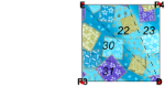
2: {20,21,28,29}

3: {16,24}
4: {36,52}
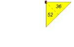
5: {37,53}
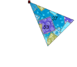
6: {17,19,25,27}

In[]:=
InsideReverseFold[{29,31},"G2D"]
Flying crane: Step 38
Out[]=

In[]:=
InsideReverseFold[{21,23},"DH2"]
Flying crane: Step 42
Out[]=

We have obtained the desired petals.
In[]:=
VFold["G2H2"]
Flying crane: Step 43
Out[]=

Leg construction
Leg construction
Right leg
Right leg
Flying Crane: Step 48
In[]:=
HO["F2C","F2I"]
Flying crane: Step 48
Out[]=
 ,
,
In[]:=
HO[FoldLine->1,Mark->{{"RC","V","v2","v3","v4"}},Handle->"A"]!
Flying crane: Step 50
Out[]=

In the next step, we apply an inside-reverse fold to the right leg part to lift it. The argument of command InsideReverseFold is hard to prepare by looking at the visible faces of from above. We have to find the middle face layer in the stack of face layers. To see the inside of the origami , we invoke command ShowLayeredFace with BaseView->True. The view of the whole origami helps identify each piece of the face.
O
50
O
50
Expand the following cell to see the output.
In[]:=
Block[{$showLayeredFace=True},ShowLayeredFace[BaseView->True]]
In[]:=
rightabove={97,101,103,99};rightbelow={115,119,117,113};
In[]:=
InsideReverseFold[{rightbelow,rightabove},"F2V"]
Flying crane: Step 54
Out[]=

Left leg
Left leg
Similarly, we uplift the tail part to make a left leg.
In[]:=
ShowOrigami[]
Out[]=

Flying crane: Step 54
Flying crane: Step 54upg
Out[]=
In[]:=
HO["F1C","F1L"]
Flying crane: Step 54
Out[]=
In[]:=
HO[FoldLine->1,Mark->{{"LC","U","u2","u3","u4"}},Handle->"C"]!
Flying crane: Step 56
Out[]=
Expand the following cell to see the output.
In[]:=
ShowLayeredFace[BaseView->True]
In[]:=
leftabove={65,69,71,67};leftbelow={83,87,85,81};
In[]:=
InsideReverseFold[{leftbelow,leftabove},"UF1"]
Flying crane: Step 60
Out[]=

Bill construction
Bill construction
Preparation for bill construction
Preparation for bill construction
Let us examine the current origami by command ShowOrigami. It displays the origami only with points specified by named parameter MarkPoints. Points U and V mark the corners of wings and legs.
In[]:=
ShowOrigami[MarkPoints->{"A","C","U","V"}]
Flying crane: Step 60
Out[]=

To make the crane bill on the right-side leg, we will put a pair of points on each edge of the lifted leg. To locate the positions of the pair of points on each edge, we use the geometric algebra g3 \cite{hestenes : 1986, Ida:2016}. A Mathematica implementation of g3 is, by default, included in Eos. In g3, a point is realized as a 1-vector. Since we often need the position of a point, we use a location vector, i.e., the starting point of a vector is the origin of the underlying coordinate system. We use NewVec command to create a 1-vector from a point. We define three 1-vector vA, vF2, and vV corresponding to points A, F2, and V, respectively.
In[]:=
vA=NewVec["A"];vF2=NewVec["F2"];vV=NewVec["V"];
G3Lineine[X, Y] [t] defines a directed line in parameter t that passed through points V and A. G3Line is defined in the package g3.
In[]:=
aline=G3Line[{vV,vA}];bline=G3Line[{vF2,vA}];
NewVec[P-> V], where P is a point name and V is a 1-vector associates P with V.
In[]:=
NewVec["Z1"->aline[0.7]];
In[]:=
NewVec["Z2"->bline[0.65]];
Here the values 0.7 and 0.65 are arbitrary, as long as Z1Z2 defines the segment along which we can fold to make the bill of the crane .
In[]:=
ShowOrigami[ImageSize->300]
Flying crane: Step 60
Out[]=

We make crease Z1Z2 to prepare for command InsideReverseFold .
In[]:=
HO["Z1Z2",Handle->"A"]!
Flying crane: Step 62
Out[]=

Expand the following cell to see the output.
In[]:=
ShowLayeredFace[Level->{9,10,11,12,13,14,15,16}]
In[]:=
above={411,403,387}
Flying crane: Step 62
Out[]=
{411,403,387}
In[]:=
above={199,207,203,195};
In[]:=
below={227,235,239,231};
In[]:=
InsideReverseFold[{below,above},"Z1Z2"]
Flying crane: Step 66
Out[]=

In[]:=
ShowOrigami[ImageSize->300]
Flying crane: Step 66
Out[]=

At this point, we could say that we have completed the construction of a flying crane origami. We can open both the wings outwards so that it looks like flying. However, as a renowned physicist K. Fushimi, who also took an interest in origami, remarked, the elegance and the simplicity of traditional origami come partly from the property that many origami artworks are flat, i.e., a stack of bounded planes.
We keep going further and open the wings.
Wing construction
Wing construction
ShowLayeredFace[BaseView->True](*outputisavailableinthefullnotebook*)
In[]:=
FO[-(3/8)π][{38,68,54,100},"IJ"]
Flying crane: Step 67
Out[]=

In[]:=
ShowOrigami[ImageSize->300,Gap->0.01]
Flying crane: Step 67
Out[]=

In[]:=
TurnOver[3]
Flying crane: Step 68
Out[]=

In[]:=
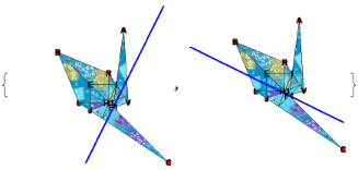
FO[-(3/8)π]["JI"]
Flying crane: Step 69
Out[]=

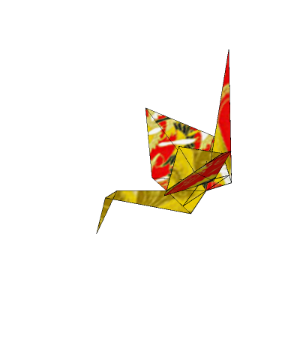
Now we complete the construction. We can display origami with different appearances by command ShowOrigami[i]. In addition to argument i, it accepts most of Mathematica’s graphics3D named parameters and the named parameters of Orikoto. For example, argument ImageSize changes the size of the graphics output, and Gap changes the spacing between the superposing layers of face stacks.
O
i
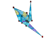
In[]:=
ShowOrigami[ImageSize->300,Gap->0.01]
Flying crane: Step 69
Out[]=

Furthermore, we can omit displaying mark points and face Ids.
In[]:=
ShowOrigami[ImageSize->300,Gap->0.001,MarkPoints->{},ShowFrame->False]
Flying crane: Step 69
Out[]=

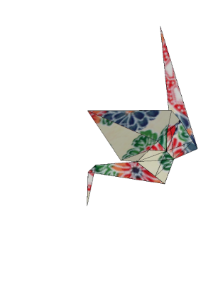
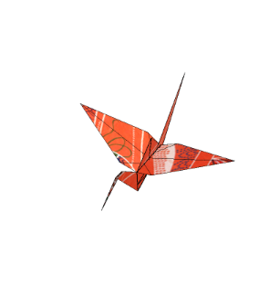
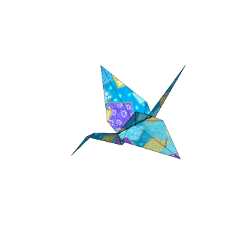
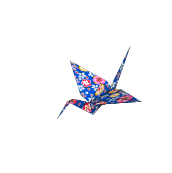
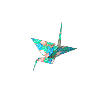
5. Texture Variations
5. Texture Variations
With another pattern of textures, we can generate various flying cranes. We do not have to change the values of parameters, such as the coordinate of the points. We have only three free parameters in this construction.
During evaluation of In[]:=

During evaluation of In[]:=

During evaluation of In[]:=

During evaluation of In[]:=

During evaluation of In[]:=

During evaluation of In[]:=

During evaluation of In[]:=

During evaluation of In[]:=

6. Concluding remarks
6. Concluding remarks
This post has shown an application of Eos-implementation of classical origami “flying crane.” Eos (E-origami system) extensively uses Mathematica’s powerful symbolic, algebraic, and graphics capabilities. We use the new modeling of origami described in our article \cite{ida:2021}. By introducing operations of cutting and gluing the edges of origami faces, we can clarify the notion of fold in classical origami. We provide new functions that simulate classical folds. Those functions are implemented in Mathematica \cite{wolfram:2022} They will be available to Mathematica programmers.
Acknowledgements
Acknowledgements
This work is supported by JSPS research grant Kakenhi 16K00008.
BibTex Reference
BibTex Reference
1
.@book {hestenes : 1986, author = {{D . Hestenes}}, publisher = {Kluwer Academic Publishers}, title = {New Foundations for Classical Mechanics (Second Edition)}, year = {1986}}
2
.@inproceedings {Ida : 2016, address = {Strasbourg, France}, author = {T . Ida and J . Fleuriot and F . Ghourabi}, booktitle = {Proceedings of ADG 2016 : The 11 th International Workshop on Automated Deduction in Geometry}, date - modified = {2018 - 03 - 16 07 : 35 : 46 + 0000}, editor = {J . Narboux and P . Schreck and I . Streinu}, month = {June}, pages = {117-- 136}, title = {A New Formalization of Origami in Geometric Algebra}, year = {2016}}
3
.@inproceedings {Huzita : 1989 a, address = {Ferrara, Italy}, author = {H . Huzita}, booktitle = {Proceedings of the First International Meeting of Origami Science and Technology}, editor = {H . Huzita}, month = {December}, pages = {143-- 158}, title = {Axiomatic Development of Origami Geometry}, year = {1989}}
4
.@inproceedings {Justin : 1989, address = {Ferrara, Italy}, author = {J . Justin}, booktitle = {Proceedings of the First International Meeting of Origami Science and Technolog}, editor = {H . Huzita}, month = {December}, pages = {251-- 261}, title = {R {\' e} solution par le pliage de l' {\' e} quation du 3 e degr {\' e} et applications g {\' e} om {\' e} triques}, year = {1989}}
5
.@inproceedings {ida : 2021, author = {T . Ida and H . Takahashi}, booktitle = {Proceedings of the 13 th International Conference on Automated Deduction in Geometry}, editor = {P . Jani {\v c} i {\' c} and Z . Kov {\' a} cs}, month = {September}, number = {352}, publisher = {Elsevier Inc .}, series = {EPTCS}, title = {A new modeling of classical folds in computational origami}, volume = {352}, year = {2021}}
6
.@book {ida : 2020, author = {T . Ida}, month = {September}, publisher = {Springer International Publishing Switzerland}, series = {Texts and Monographs in Symbolic Computation}, title = {An introduction to Computational Origami}, year = {2020}}
7
.@misc {wolfram : 2022, author = {{Wolfram Research {, } Inc .}}, title = {Mathematica}, year = {2022}}
CITE THIS NOTEBOOK
CITE THIS NOTEBOOK
A new modeling of classical folds in computational origami
by Tetsuo Ida, Hidekazu Takahashi
Wolfram Community, STAFF PICKS, June 16, 2022
https://community.wolfram.com/groups/-/m/t/2551017
by Tetsuo Ida, Hidekazu Takahashi
Wolfram Community, STAFF PICKS, June 16, 2022
https://community.wolfram.com/groups/-/m/t/2551017