Introduction
Disclaimer : I am an ARM employee but this is a personal work.
I wanted to understand how to convert a Neural network from Mathematica to use it on a Cortex-M with the CMSIS-NN library. CMSIS-NN is a free ARM library containing a few optimized functions for Neural networks on embedded systems (convolutional layers and fully connected).
There are a few demos (CIFAR and Keyword spotting) running on Cortex-M. There were generated either from Caffe framework or with TensorFlow Lite.
I wanted to do the same from Mathematica and also understand a bit more the CMSIS-NN library. So, I attempted to reproduce a keyword spotting example.
CMSIS-NN is part of the CMSIS library which can be downloaded here: https://github.com/ARM-software/CMSIS_5
The keyword spotting example was used.
Keyword Spotting
Keyword Spotting
The keyword spotting on microcontroller use case is described in this article: https://arxiv.org/pdf/1711.07128.pdf
Some example code can be found here : https://github.com/ARM-software/ML-KWS-for-MCU
Keyword spotting test patterns can be downloaded from here :
http://download.tensorflow.org/data/speech_commands_v0.02.tar.gz
http://download.tensorflow.org/data/speech_commands_v0.02.tar.gz
The network used in this document is close but different from the networks you’ll find in previous link. Also we are not implementing the full demo but just experimenting about how to use CMSIS-NN with Mathematica.
The Network
The Network
The network is quite simple but for an embedded system we cannot use something too complex. First the audio is going through a MFCC step:
audioEnc=NetEncoder[{"AudioMFCC","WindowSize"->4*160,"Offset"->2*160,"NumberOfCoefficients"->10,"TargetLength"->49,SampleRate->16000}]
The network is standard : a few convolutional layers followed by a few fully connected layers:
kwsModel=NetChain[{ReplicateLayer[1],ConvolutionLayer[channels[[1]],{10,4}],ElementwiseLayer[Ramp],ConvolutionLayer[channels[[2]],{10,4},"Input"->{channels[[1]],40,7},"Stride"->{2,1}],ElementwiseLayer[Ramp],LinearLayer[58],ElementwiseLayer[Ramp],LinearLayer[128],ElementwiseLayer[Ramp],LinearLayer[Length[wantedClass]],SoftmaxLayer[]},"Input"->audioEnc,"Output"->classDec]
At the output, there is a NetDecoder which is converting the output into 3 classes. I am trying to detect the word “backward”, “yes”, “no”.
The test patterns are coming from the TensorFlow keyword spotting example (link in attached notebook). But my network is different.
The test patterns are coming from the TensorFlow keyword spotting example (link in attached notebook). But my network is different.
Problems to solve
Problems to solve
There are 2 problems to solve to be able to convert this network for CMSIS-NN.
First problem : the library is using a different convention for the tensors which means that the weights have to be reordered before being used by CMSIS-NN. Since it is not too difficult to do with Mathematica, I won’t detail it here.
Second problem : CMSIS-NN is using fixed point arithmetic (Q15 or Q7). But Mathematica is using float. Two limitations of Mathematica : there are no quantization operators so we cannot learn the network with the quantization effects. It is not a major issue but we can expect that the quantized network will be less good than if we had trained directly with quantization effects.
Second limitation : During training Mathematica is not keeping track of the statistics of the intermediate values (input and output of layers). But to convert the float into fixed point we need to know some statistics about the dynamic of those values. Once the dynamic is known, the quantization is controlled with parameters of the CMSIS-NN layers : shift values for the weight and bias.
So, to get those statistics I am just applying each layer of the trained network one after another and keeping track of the input / output. I do this on all training patterns. By luck embedded networks are small so even if it is slow to do this, it is not too slow.
I get beautiful histograms (log scale) which are used as a basis to choose how to quantize the values. A simple strategy is to just use the min and max values.
Code generation
Code generation
Once I have statistics for the dynamics of the values, I can generate C code for CMSIS-NN and C arrays containing the quantized values.
Since quantization has an effect on the performance of the network, I want to be able to test the result easily. So, I have customized CMSIS-NN to be able to run it from Mathematica. The C code generated by the Notebook can be compiled and used with Mathlink.
Like that I can compare the behavior of the original network and the CMSIS-NN quantized one. Here is an example:
To use the notebook
To use the notebook
The steps to convert a network are:
◼
Train a network
◼
Compute statistics on the network intermediate values
netStats=ComputeAllFiles[result,audioEnc,trainingFiles,SumStat];
result is the trained network.
audioEnc is the MFCC
trainingFiles are the training files.
SumStat is the strategy used for the statistics. Here we just get a summary statistics : just min/max
audioEnc is the MFCC
trainingFiles are the training files.
SumStat is the strategy used for the statistics. Here we just get a summary statistics : just min/max
◼
Quantize the network and generate C code
mfcc=audioEnc[AudioResample[SpeechSynthesize["backward"],16000]];quantizedNetwork1=CorrectedFormats[result,netStats,15,0];quantizedNetwork=<|"w"->quantizedNetwork1["w"],"net"->Drop[quantizedNetwork1["net"],1]|>;TestPatterns[NetDrop[result,1],NetExtract[result,1][mfcc],quantizedNetwork];CompileNetwork[NetDrop[result,1],NetExtract[result,1][mfcc],result[mfcc,None],quantizedNetwork]TestCode[NetDrop[result,1],quantizedNetwork];
In this example NetDrop is just dropping the first ReplicateLayer. It does not exist in CMSIS-NN and it is used here just to adapt the tensor shape at the input of the network.
The second and third arguments of CompileNetwork are input and output of the network on one test pattern. It is used only when debugging the network.
mfcc is the input pattern (mfcc of some audio pattern).
◼
Compiling the generated code in ctests using the provided Makefile
◼
Linking the executable and start using it
link=Install[FileNameJoin[{NotebookDirectory[],"ctests","cmsisnn.exe"}]];cmsiskws[s_]:=classDec[CMSISNN[QuantizeData[15,quantizedNetwork["net"][[1,2]],Transpose[audioEnc[s]//ReplicateLayer[1],{3,2,1}]//Flatten]]];
The cmsiskws is a convenience function. It is quantizing the input data using the format computed during quantization of the network.
Then it is computing the MFCC of the audio, reordering the data (Transpose) to use the same convention as CMSIS-NN. Then the CMSISNN function is called on the result.
cmsiskws[AudioResample[SpeechSynthesize["yes"],16000]]
We can now test that this C code can recognize the word “yes”.
The same notebook and same principles were used on CIFAR example.
The same notebook and same principles were used on CIFAR example.
Code and details
Data processing
Data processing
The first step in any neural network work is to get some data to train, validate and test the network. Often the data is not in the format required by the framework and some pre-processing and converting work is required.
In this example we are using the test patterns from the tensorflow keyword spotting example. But, we are not going to apply the noise patterns and we are going to restrict the training to only a subset of the keywords. So we are simplifying the problem.
Paths
Paths
In[]:=
(*LocationofthefoldercontainingtheKWStestpatterns*)patterndir="C:\\MachineLearningTests\\data_speech_commands_v0.02";
In[]:=
(*Wheretoserializethetrainednetwork*)traineddir=FileNameJoin[{NotebookDirectory[],"trainedNetworks"}];CreateDirectory[traineddir];
Pre-processing functions
Pre-processing functions
List of keywords
List of keywords
The keywords we have selected for use in the test:
In[]:=
wantedClass={"yes","no","backward"};
Scan all directories to extract the file names corresponding to the wantedClass and not in the background noise folder
In[]:=
(*Listofallexistingkeywordsinthefolderwithoutthenoisefolder*)allClasses=Select[FileNameTake[#,-1]&/@Select[FileNames[patterndir<>"\\*"],DirectoryQ],#!="_background_noise_"&];
Test files
Test files
Test patterns
Test patterns
Network and Network Training
Network and Network Training
Audio encoder
Audio encoder
The audio files are passed through an audio encoder (Mathematica terminology) which is extracting features. The network is trained on those features. MFCC is used. In a real application you would have to use the MFCC from your board which could be implemented for instance with CMSIS-DSP (a library of DSP functions optimized for Cortex-M).
In[]:=
audioEnc=NetEncoder[{"AudioMFCC","WindowSize"4*160,"Offset"2*160,"NumberOfCoefficients"10,"TargetLength"49,SampleRate16000}]
Out[]=
NetEncoder

Class decoder
Class decoder
In a similar way, the output of the network is going through a network decoder to display a class.
In[]:=
classDec=NetDecoder[{"Class",wantedClass}]
Out[]=
NetDecoder
Network sizing
Network sizing
Different sizes can be used for the layer of the network. 3 possible configurations are defined here and the first one is used. Those configurations are coming from the C implementation where 3 possible configurations are defined in header files.
In[]:=
channels1={28,30};channels2={64,48};channels3={60,76};channels=channels1;
Network definition
Network definition
The definition of a network for keyword spotting. Compared to the C version, the only difference is the softmax layer at the end.
In[]:=
kwsModel=NetChain[{ReplicateLayer[1],ConvolutionLayer[channels[[1]],{10,4}],ElementwiseLayer[Ramp],ConvolutionLayer[channels[[2]],{10,4},"Input"->{channels[[1]],40,7},"Stride"{2,1}],ElementwiseLayer[Ramp],LinearLayer[58],ElementwiseLayer[Ramp],LinearLayer[128],ElementwiseLayer[Ramp],LinearLayer[Length[wantedClass]],SoftmaxLayer[]},"Input"audioEnc,"Output"classDec]
Out[]=
NetChain
Network training
Network training
Training the kws network with the defined training patterns and the validation patterns. The validation patterns are used to avoid overfitting. Test patterns are needed after to test the trained network
In[]:=
trainedModel=NetTrain[kwsModel,trainingPatterns,All,ValidationSetvalidationPatterns]
Out[]=
Training a network takes time. So the trained network is serialized to disk.
In[]:=
DeleteFile[FileNameJoin[{traineddir,"trained"}]];Save[FileNameJoin[{traineddir,"trained"}],trainedModel]
When needed, the network can be restored from drive. The variable trainedModel will be recreated.
In[]:=
ClearAll[trainedModel];Get[FileNameJoin[{traineddir,"trained"}]];

From this trained network, we extract only the inference engine (and not the additional data about the training errors):
The trained network
The trained network
trainedModel is containing lot of information about the training like final error, evolution of error during training etc ... Here, we extract the trained network to use it.
In[]:=
result=trainedModel["TrainedNet"];
It is this result variable that will be used in other parts of the document to use the network.
Network Testing
Network Testing
To test the network, we can compute some statistics or play with it.
Performance statistics
Performance statistics
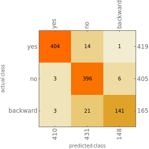
The statistics are computed on the test patterns. It is useful to see how the network is behaving on patterns it has never seen.
In[]:=
measurementsFloat=ClassifierMeasurements[result,testPatterns];
In[]:=
measurementsFloat["Accuracy"]
Out[]=
0.957533
In[]:=
measurementsFloat["ConfusionMatrixPlot"]
Out[]=
Playing with the network
Playing with the network
It is good to get an intuitive understanding of the network and for this a simple UI to play with it can be useful.
In[]:=
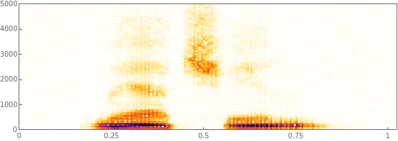
Manipulate[Module[{s,d,n,f=noiseLevel,noisy,i,rec,col},s=AudioResample[SpeechSynthesize[word],16000];d=Duration[s];n=AudioGenerator[noiseKind,d,SampleRate16000];noisy=s+f*n;rec=result[noisy];i=Spectrogram[noisy,ImageSizeLarge];col=If[recword,RGBColor[0,0.7,0],Red];Column[{Row[{"Noise Level: ",noiseLevel}],i,Row[{Text[Style["Recognized word : ",14]],Text[Style[rec,col,14]]}]}]],{noiseLevel,0.0,0.25},{noiseKind,{"White","Pink","Brown","Blue"}},{word,{"yes","no","backward","truc","machin"}},ContinuousActionFalse,SaveDefinitionsTrue]
Out[]=


◼
Fixed Point Network
CMSIS-NN
CMSIS-NN
The CMSIS - NN library is described in detail in the following document.
https://arxiv.org/abs/1801.06601
https://arxiv.org/abs/1801.06601
There are several challenge to convert a Neural Network into CMSIS-NN :
◼
Unsupported kernels
◼
Data Layout
◼
Quantization of coefficients
◼
Quantization of activations
◼
Testing the result
Unsupported Kernels
Unsupported Kernels
CMSIS-NN is only supporting small number of kernels. The network should contain only similar kernels or kernels which can be replaced with an equivalent combination of CMSIS-NN kernels. Otherwise, it won’t be possible to convert the network to CMSIS-NN.
Data Layout
Data Layout
CMSIS-NN and Mathematica are using different conventions for the tensors. So the weights must be reordered before being dumped for use with CMSIS-NN.
Since the reordering is not simple, I advise to test it with a float version of CMSIS-NN when you want to support a new kind of layer.
Note that in CMSIS-NN, there is also another reordering of the weights which is for performance purpose only and for the _opt version of the fully connected algorithms. It is separate from above problem and this other weight reordering should be applied after above reordering if the _opt functions are used.
Quantization
Quantization
The Problem
The Problem
Quantization of a network is a difficult problem. When switching from floating point to fixed point arithmetic we introduce truncation noise and saturation effects. Truncation noise is bigger in absolute value in the fixed point version since the dynamic which can be represented is smaller than with float.
There are two way to address the problem of quantizing a network:
There are two way to address the problem of quantizing a network:
◼
Training with a quantized network
◼
Quantizing an existing network
First solution is expected to give better results since the network is trained with the truncation noise and the saturation effects. But it is not supported by Mathematica. So we are going to try to quantize and existing network.
For the weights and biases, it is simple : the values are known. So you can quantize them easily and find the fixed point position allowing to map the values inside the chosen word size (word16 or word8 for CMSIS-NN).
For the activation and intermediate computations it is more difficult.
For the activation and intermediate computations it is more difficult.
Quantization of Activations
Quantization of Activations
If the quantization is only based on input / output (and not the internal of each fixed point kernel), then we only need some statistics on the input / output.
Some frameworks (TensorFlow for instance) allow to gather information about the min/max during training. It may require the introduction of special operators. But it is not supported by Mathematica. So, after the training we have to compute those statistics by applying each layer one after another.
Some frameworks (TensorFlow for instance) allow to gather information about the min/max during training. It may require the introduction of special operators. But it is not supported by Mathematica. So, after the training we have to compute those statistics by applying each layer one after another.
Once this data is available, you’re ready to quantize the network.
You know the Q format of the input, output, weight and bias. From this you can compute the bias shift and out shift needed in CMSIS-NN.
If fi is the number of fractional bits for the input, fo for the output, fw for the weight and fb for the biases then:
◼
The bias shift is : (fi + fw) - fb
◼
The out shift is : (fi + fw) - fo
For layers where there is no shift available, then the output format will be computed from the input format and the implementation details of the kernel but not from the output statistics. For instance, for a max pooling you have no choice : the output has same fixed point format as the input even if the statistics show that perhaps a better format could be chosen for the output.
So the format of the input / output of layer of a network are not just dependent on the statistics of the input / output. They also depend on how the layers are connected.
This quantization approach will not show if there can be problems during the computations. For this reason it is very important to test the final behavior of the quantized network.
Quantization schemes
Quantization schemes
How to define the Q format from the activation statistics ?
The simplest way is to get the min and the max and use it to compute the Q format.
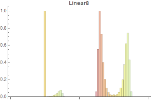
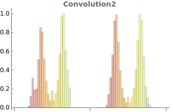
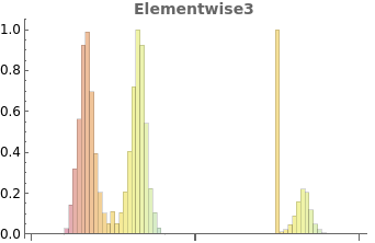
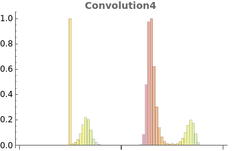
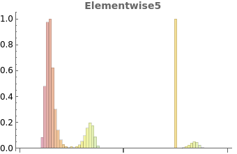
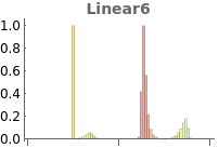
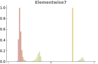
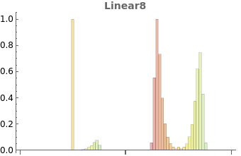
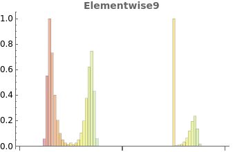
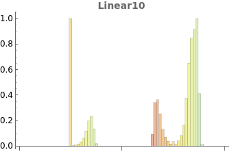
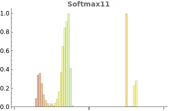
Below, some histogram of the activations of the network. On the left it is the input of a layer. On the right the output. The scale is logarithmic. It is the exponent for positive values and -exponent for negative values.
From those histograms we see that the values are often highly concentrated. So, instead of using the min / max we could decide to have saturation / sign inversion for values far from the concentrated part of the histogram and more fractional bits for the center of the histogram. It would be a different quantization scheme since the Q format would not take into account the less likely values.
In the testing section we will show results where we keep only 80% of the most likely values to do the quantization.
Code Generation
Code Generation
Network quantization utilities
Network quantization utilities
Q format
Q format
Quantization utility functions
Quantization utility functions
Quantization statistic functions
Quantization statistic functions
Utilities functions to compute activation formats of network
Utilities functions to compute activation formats of network
C file generation
C file generation
In[]:=
ctests=FileNameJoin[{NotebookDirectory[],"ctests"}];
C file generation for code and coefficients
C file generation for code and coefficients
C file generation for testing
C file generation for testing
Network compilation
Network compilation
Testing code generation
Testing code generation
Testing
Testing
Statistics computations
Statistics computations
min / max statistics computed on all training file and serialization / restoration from disk.
min / max statistics computed on all training file and serialization / restoration from disk.
In[]:=
netStats=ComputeAllFiles[result,audioEnc,trainingFiles,SumStat];
In[]:=
DeleteFile[FileNameJoin[{traineddir,"netStats"}]];Save[FileNameJoin[{traineddir,"netStats"}],netStats]
In[]:=
ClearAll[netStats];Get[FileNameJoin[{traineddir,"netStats"}]];
Histogram statistics
Histogram statistics
In[]:=
netHistStats=ComputeAllFiles[result,audioEnc,trainingFiles,HistStat];
In[]:=
DeleteFile[FileNameJoin[{traineddir,"netHistStats"}]];Save[FileNameJoin[{traineddir,"netHistStats"}],netHistStats]
ClearAll[netHistStats];Get[FileNameJoin[{traineddir,"netHistStats"}]]
Raw histograms: no statistics. They are used for graphical display or to recompute histogram statistics.
Raw histograms: no statistics. They are used for graphical display or to recompute histogram statistics.
In[]:=
histograms=ComputeAllFiles[result,audioEnc,trainingFiles,HistStat,True];
In[]:=
DeleteFile[FileNameJoin[{traineddir,"rawNetHistStats"}]];Save[FileNameJoin[{traineddir,"rawNetHistStats"}],histograms];
ClearAll[histograms];Get[FileNameJoin[{traineddir,"rawNetHistStats"}]];
Graphical display of histograms
Graphical display of histograms
In[]:=
hists=With[{maxNb=Length[histograms]},Table[DrawHist[histograms,result,i,iRound[(maxNb-2)/2+2]],{i,2,maxNb}]]
Out[]=
,
,
,
,
,
,
,
,
,
Float example
Float example
Float implementation of CMSIS-NN to validate the weight reordering functions. It is generating the float version of the code and the test code and test patterns. Then it can be launched from command line to test if there are errors.
The Makefile must be used to compile the TestCode.
The Makefile must be used to compile the TestCode.
In[]:=
mfcc=audioEnc[AudioResample[SpeechSynthesize["yes"],16000]];(*Forinputpatternweuseoutputofreplicatelayer.Wedropthenetdecoderattheend*)CompileNetwork[NetDrop[result,1],NetExtract[result,1][mfcc],result[mfcc,None],f32](*Fortestpatternswedropthereplicatelayer*)TestPatterns[NetDrop[result,1],NetExtract[result,1][mfcc],f32]TestCode[NetDrop[result,1],f32];
Fixed point example
Fixed point example
Here the normal stats are used. netHistStats could be used too to get the histogram based quantization. MakefileMath.make must be used to be able to call the C network from Mathematica.
In[]:=
mfcc=audioEnc[AudioResample[SpeechSynthesize["backward"],16000]];quantizedNetwork1=CorrectedFormats[result,netStats,15,0];quantizedNetwork=<|"w"quantizedNetwork1["w"],"net"Drop[quantizedNetwork1["net"],1]|>;TestPatterns[NetDrop[result,1],NetExtract[result,1][mfcc],quantizedNetwork];CompileNetwork[NetDrop[result,1],NetExtract[result,1][mfcc],result[mfcc,None],quantizedNetwork]TestCode[NetDrop[result,1],quantizedNetwork];
Comparing float and q15 format
Comparing float and q15 format
Here the C network is going to be called from Mathematica and compared to the Mathematica network.
Wrapper for C version of the network
Wrapper for C version of the network
The function is taking as input a sound and converting it into a form which can be processed by the C version.
So sound is encoded using audioEnc (mfcc), then the data is reordered to correspond to the CMSIS ordering, then they are quantized based upon input network statistics and in Q15. If a Q7 version was used, this function would have to be changed or get the word size from quantizedNetwork instead of hardcoding it here.
So sound is encoded using audioEnc (mfcc), then the data is reordered to correspond to the CMSIS ordering, then they are quantized based upon input network statistics and in Q15. If a Q7 version was used, this function would have to be changed or get the word size from quantizedNetwork instead of hardcoding it here.
In[]:=
ClearAll[cmsiskws];cmsiskws[s_]:=classDec[CMSISNN[QuantizeData[15,quantizedNetwork["net"][[1,2]],Transpose[audioEnc[s]//ReplicateLayer[1],{3,2,1}]//Flatten]]];
Connection to the C version
Connection to the C version
If the C has been compiled with the right Makefile then, communication with Mathematica can be started with next line. The C is launched in another process and communicate with Mathematica.
In[]:=
link=Install[FileNameJoin[{NotebookDirectory[],"ctests","cmsisnn.exe"}]];
Following line can be used to check everything is working and C code is exporting CMSISNN to Mathematica.
In[]:=
LinkPatterns[link]
Out[]=
{CMSISNN[i_List]}
Following line can be used to make a quick tests and see if the “yes” keyword is recognized by the C network. The speech synthetizer is not using the right sampling rate. The network was trained with 16 kHz sampling rate. So, we resample the speech before using the network.
In[]:=
cmsiskws[AudioResample[SpeechSynthesize["yes"],16000]]
Out[]=
yes
UI to play with float and fixed point version
UI to play with float and fixed point version
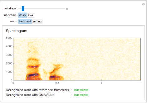
A simple UI is built to play with the network and compare it to the Mathematica reference. It will only work if the cmsisnn.exe has been “linked” to Mathematica.
comp=Manipulate[With[{textSize=14},Module[{s,d,n,f=noiseLevel,noisy,i,rec,col,fixedfrec,colrec},s=AudioResample[SpeechSynthesize[word],16000];d=Duration[s];n=AudioGenerator[noiseKind,d,SampleRate16000];noisy=s+f*n;rec=result[noisy];fixedfrec=cmsiskws[noisy];i=Spectrogram[noisy,ImageSizeLarge,LabelStyleDirective[FontSize12]];col=If[recword,RGBColor[0,0.7,0],Red];colrec=If[fixedfrecword,RGBColor[0,0.7,0],Red];Column[{Text[Style["Spectrogram",16]],(*Row[{"Noise Level: ",noiseLevel}],*)i,Grid[{{Text[Style["Recognized word with reference framework",textSize]],Text[Style[":",textSize]],Text[Style[rec,col,textSize]]},{Text[Style["Recognized word with CMSIS-NN",textSize]],Text[Style[":",textSize]],Text[Style[fixedfrec,colrec,textSize]]}},Alignment{Left,Baseline}]},Spacings1]]],{{noiseLevel,0.02},0.0,0.25},{noiseKind,{"White","Pink"}},{word,{"backward","yes","no"}},ContinuousActionFalse,LabelStyleDirective[FontSize12]]
Function for computing accuracy of fixed point version
Function for computing accuracy of fixed point version
Accuracy of different fixed point versions
Accuracy of different fixed point versions
Accuracy tested with normal stats.
Accuracy tested with normal stats.
In[]:=
FixedAccuracy[cmsiskws,testPatterns]
Out[]=
0.874621
Accuracy with histogram quantization : A new C code must be generated and recompiled before testing it.
Accuracy with histogram quantization : A new C code must be generated and recompiled before testing it.
In[]:=
FixedAccuracy[cmsiskws,testPatterns]
Out[]=
0.82002
Disconnection from the C code. Must be done before trying to recompile the C code.
In[]:=
Uninstall[link]
Out[]=
"C:\MachineLearningTests\ForWolframForum\ctests\cmsisnn.exe"
Conclusion
It works but it is not a real application.
The network was trained with the Mathematica MFCC. In a real application you would need to train with the MFCC you use on your board.
Also, we are using a short segment from the audio. In a real application you would need to take into account the fact that words have different lengths.
Finally, in the audio the word to recognize may be anywhere so a kind of sliding window would have to be used and the recognition applied on all the windows.
Finally, in the audio the word to recognize may be anywhere so a kind of sliding window would have to be used and the recognition applied on all the windows.
In a real application you would try to reuse the working buffers as much as possible to minimize memory usage. It is not done by the code generation here.
Finally, in CMSIS-NN there are often different versions of the same layer. For instance a square and non-square version. The code generation of this notebook is always using the most generic and not the most efficient.
Finally, in CMSIS-NN there are often different versions of the same layer. For instance a square and non-square version. The code generation of this notebook is always using the most generic and not the most efficient.
So, the C code generated by this Notebook would have to be modified a little bit before being used in a real embedded application.