This is part of live presentation series called Mathematical Games in which we explore a variety of games and puzzles using Wolfram Language. In this episode, we feature games and puzzles focusing on Linear Algebra magic.
demonstrations.wolfram.com
demonstrations.wolfram.com
Rotating a Tetrahedron
Rotating a Tetrahedron
Here’s a tetrahedron that I will rotate. How many applications of linear algebra are there?
In[]:=
PolyhedronData["Tetrahedron"]
Out[]=

Tentative list of the Linear Algebra Involved
Tentative list of the Linear Algebra Involved
3D Point Representation
3D Point Representation
Mouse Movement Vectors
Mouse Movement Vectors
Matrix Transformation: Rotation matrix
Matrix Transformation: Rotation matrix
Vector Representation: Representing the vertices, edges and faces
Vector Representation: Representing the vertices, edges and faces
Homogeneous Coordinates: handle translations and rotations
Homogeneous Coordinates: handle translations and rotations
Dot Product: Calculating angles between vectors to determine the direction and magnitude of rotation.
Dot Product: Calculating angles between vectors to determine the direction and magnitude of rotation.
Cross Product: Finding the axis of rotation by determining the perpendicular vector to the plane formed by the initial and final positions.
Cross Product: Finding the axis of rotation by determining the perpendicular vector to the plane formed by the initial and final positions.
Projection: Using projection matrices to convert 3D coordinates to 2D screen coordinates for rendering.
Projection: Using projection matrices to convert 3D coordinates to 2D screen coordinates for rendering.
Normal Vectors: Calculating normal vectors for the faces of the tetrahedron to determine their orientation relative to light sources and the camera.
Normal Vectors: Calculating normal vectors for the faces of the tetrahedron to determine their orientation relative to light sources and the camera.
Barycentric Coordinates: Using barycentric coordinates for interpolation within the tetrahedron’s faces, useful for texture mapping or shading.
Barycentric Coordinates: Using barycentric coordinates for interpolation within the tetrahedron’s faces, useful for texture mapping or shading.
Camera Transformations: Applying view matrices to simulate the camera’s position and orientation in the scene.
Camera Transformations: Applying view matrices to simulate the camera’s position and orientation in the scene.
Clipping: Performing clipping operations to handle parts of the tetrahedron that are outside the view frustum.
Clipping: Performing clipping operations to handle parts of the tetrahedron that are outside the view frustum.
Interpolation: Interpolating between keyframes if there is animation in the rotation or other transformations.
Interpolation: Interpolating between keyframes if there is animation in the rotation or other transformations.
Inverse Matrices: Calculating inverse matrices for undoing transformations or for certain types of error corrections and collision detections.
Inverse Matrices: Calculating inverse matrices for undoing transformations or for certain types of error corrections and collision detections.
Digital Encoding of voice and graphics
Digital Encoding of voice and graphics
Error Correction of digital data
Error Correction of digital data
Reassembly of digital data
Reassembly of digital data
Conversion of digital data into video and sound
Conversion of digital data into video and sound
Vector AB
Vector
AB
A vector from a point A to a point B is represented as .A pair of numbers such as {3,4} can represent a vector.The same vector could be a scalar distance 5 and a unit direction .
AB
,
3
5
4
5
In[]:=
Norm,
3
5
4
5
Out[]=
1
In[]:=
Norm[{3,4}]
Out[]=
5
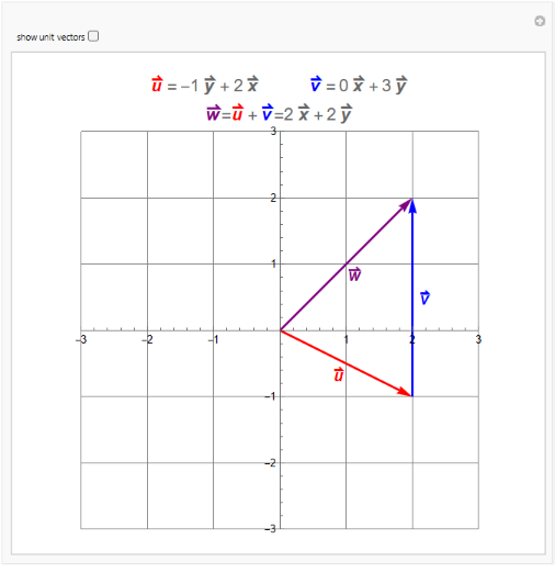
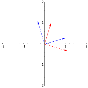
2D Vector Addition
2D Vector Addition
by: Joe Bolte
Drag the heads of the red and blue vectors to change them. The purple vector is their sum. https://demonstrations.wolfram.com/2DVectorAddition/
Kirkman Schoolgirl Problem 1850
Kirkman Schoolgirl Problem 1850
Fifteen young ladies in a school walk out three abreast for seven days in succession: it is required to arrange them daily so that no two shall walk twice abreast.
In 1850, Cayley solved the problem first. In White is a Room Square.
1. All possible pairs from 1-8 are given.
2. All digits 1-8 appear in each row and column.
1. All possible pairs from 1-8 are given.
2. All digits 1-8 appear in each row and column.
Out[]=
a | b | c | d | e | f | g | |
abc | 35 | 17 | 28 | 46 | |||
ade | 26 | 48 | 15 | 37 | |||
afg | 13 | 57 | 68 | 24 | |||
bdf | 47 | 16 | 38 | 25 | |||
bge | 58 | 23 | 14 | 67 | |||
cdg | 12 | 78 | 56 | 34 | |||
cef | 36 | 45 | 27 | 18 |
In 1850, Cayley combined a Fano Plane and a Room Square to solve the Kirkman problem.
Note: Gino Fano (5 January 1871 – 8 November 1952).
Note: Thomas Gerald Room (10 November 1902 – 2 April 1986).
Note: Gino Fano (5 January 1871 – 8 November 1952).
Note: Thomas Gerald Room (10 November 1902 – 2 April 1986).
Sylvester and Cayley solved other tricky problems with grids of numbers.
Enter the Matrix 1850 (Sylvester and Cayley)
Enter the Matrix 1850 (Sylvester and Cayley)
“For this purpose we must commence, not with a square, but with an oblong arrangement of terms consisting, suppose, of m lines and n columns. This will not in itself represent a determinant, but is, as it were, a Matrix out of which we may form various systems of determinants by fixing upon a number p, and selecting at will p lines and p columns, the squares corresponding of pth order.”
A sample matrix:
In[]:=
MatrixForm[{{1,2},{3,4}}]
Out[]//MatrixForm=
1 | 2 |
3 | 4 |
Sylvester also named Graphs.
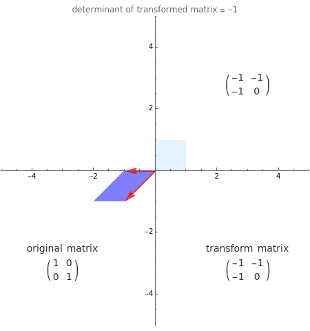
Visualizing Matrix Bases and Transforms
Visualizing Matrix Bases and Transforms
by: Roger J. Brown
There are =81 transformations that can be produced using matrices with just the three integers . Some 33 of these are degenerate, in that the transformed matrix loses a dimension and has a zero determinant. This Demonstration considers all of these cases, initially with the unit matrix as the base to be transformed. Transform number 69 is the identity matrix and number 53 is its transpose, the antidiagonal matrix.
2×2
3
2×2
{-1,0,1}
Out[]=


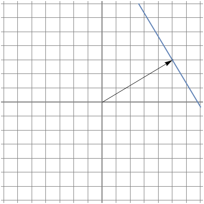
From Vector to Line
From Vector to Line
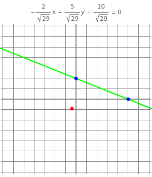
Any nonzero 2D vector defines a unique perpendicular line in 2D. Except for lines through the origin, every line defines a nonzero vector. Hover over the blue line to see the equation of the line generated by the movable point.
Out[]=
Normed Line
Normed Line
The normed version of a line is , where the point is on the unit circle. Drag a blue point to obtain a new line.
Ax+By+C=0
(A,B)
Out[]=
From Vector to Plane
From Vector to Plane
Any nonzero 3D vector defines a unique plane in 3D. Except for planes through the origin, every plane is defined by a unique vector. This vector is normal (perpendicular) to the plane. In the equation of the plane , with as the defining vector, , which is the square of the norm (length) of the vector.
Ax+By+Cz=D
(A,B,C)
D=++
2
A
2
B
2
C
In[]:=
Clear[a]
Out[]=

Three Points Determine a Hessian Plane
Three Points Determine a Hessian Plane
Three noncollinear points in three dimensions determine a unique plane with an equation of the form , where ++1 and is the positive distance of the plane from the origin. The vector is normal (perpendicular) to the plane and has norm (length) equal to 1.
Ax+By+Cz=D
2
A
2
B
2
C
D
(A,B,C)
For such an equation, the signed distance from a point to the plane is given by . Points on the same side of the plane have the same sign.
(x,y,z)
(A,B,C,D)·(x,y,z,-1)
Out[]=

The plane through three points is sometimes called the Hessian plane.
dill=RandomReal[{0,1},{3,3}];ResourceFunction["HessianPlane"][dill]
Out[]=
{-0.409554,0.364596,0.836263,0.211657}
Marianne Olympics 2024 Logo
Marianne Olympics 2024 Logo
Let’s look at the 2024 Olympics logo. The main part uses 34 points.
In[]:=
flame=;lips={{170.3`,131.4`},{168.9`,131.9`},{166.5`,132},{164.4`,130.3`},{162.4`,132},{160,131.9`},{158.5`,131.4`},{157.3`,131},{156.4`,130.7`},{154.6`,130.7`},{157.2`,125.3`},{163.7`,123},{169.1`,125.6`},{171.3`,126.7`},{173.1`,128.5`},{174.2`,130.7`},{172.5`,130.7`},{171.5`,131},{170.3`,131.4`}};Graphics,FilledCurve[{{{1,4,3},{1,3,3},{1,3,3},{1,3,3},{1,3,3},{1,3,3},{1,3,3},{1,3,3},{1,3,3},{1,3,3},{1,3,3}}},{flame}],FilledCurve[{{{1,4,3},{1,3,3},{1,3,3},{1,3,3},{1,3,3},{1,3,3}}},{lips}],Black,ResourceFunction["NumberedPointPlot"][flame][[1]],Gray,ResourceFunction["NumberedPointPlot"][lips][[1]]
Out[]=
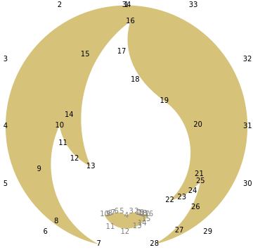
Points {1,4,7,10,13,16,19,22,25,28,31,34} are endpoints of arcs.
These points are controls for Bézier curves, first developed by French mathematician Paul de Casteljau for French automaker Citroën, but later independently developed by French engineer Pierre Bézier for French automaker Renault. These are very French curves in the Logo.
These points are controls for Bézier curves, first developed by French mathematician Paul de Casteljau for French automaker Citroën, but later independently developed by French engineer Pierre Bézier for French automaker Renault. These are very French curves in the Logo.
In[]:=
Graphics[{BezierCurve[Take[flame,{10,13}]],BezierCurve[Take[flame,{13,16}]],BezierCurve[Take[flame,{16,19}]],BezierCurve[Take[flame,{19,22}]],BezierCurve[Take[flame,{22,25}]]}]
Out[]=
In[]:=
Graphics[{BSplineCurve[Take[flame,{10,13}]],BSplineCurve[Take[flame,{13,16}]],BSplineCurve[Take[flame,{16,19}]],BSplineCurve[Take[flame,{19,22}]],BSplineCurve[Take[flame,{22,25}]]}]
Out[]=

Out[]=
Here’s one section where the de Casteljau algorithm is used to generate the points:
In[]:=
Graphics[{BezierCurve[Take[flame,{22,25}]],Point[Table[((flame[[22]](1-a)+flame[[23]]a)(1-a)+(flame[[23]](1-a)+flame[[24]]a)(a))(1-a)+((flame[[23]](1-a)+flame[[24]]a)(1-a)+(flame[[24]](1-a)+flame[[25]]a)(a))(a),{a,0,1,.05}]]}]
Out[]=
You can learn more about Bézier curves with the Demonstrations at the link Bezier. For example, Rational Cubic Bézier Curves.
Normalizing Vectors
Normalizing Vectors
by: George Beck
A nonzero vector is normalized by dividing it by its length. The resulting vector has length 1 and lies in the same direction.In 2D, the length of is given by Pythagoras’s formula: . In 3D, the length of is .In any dimension, the normalized vector of is .
v=(x,y)
|v|=+
2
x
2
y
v=(x,y,z)
|v|=++
2
x
2
y
2
z
v
v/|v|=v
v·v
Out[]=
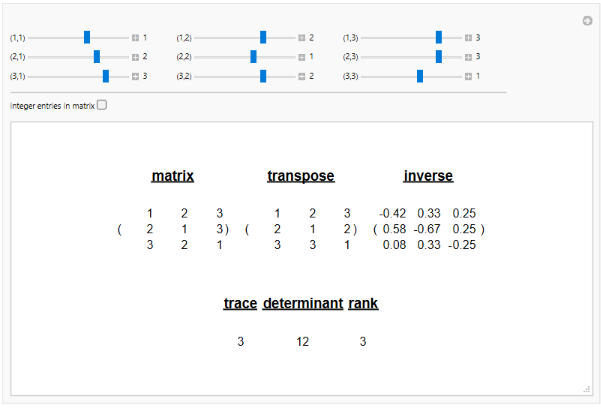
3x3 Matrix Transpose, Inverse, Trace, Determinant and Rank
3x3 Matrix Transpose, Inverse, Trace, Determinant and Rank
by: Chris Boucher
There is a natural way to generate the binary Golay code. Just use a binary factor of +1! It’s that easy!
23
x
2D Rotation Using Matrices
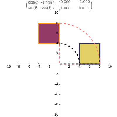
2D Rotation Using Matrices
This Demonstration illustrates the concept of rotating a 2D polygon. The rotation matrix is displayed for the current angle. The default polygon is a square that you can modify.
Out[]=
Three Parametrizations of Rotations
Three Parametrizations of Rotations
A rotation can be parameterized in several ways. This Demonstration compares three popular parametrizations:
• Euler angles about the axes
• the angle of rotation about an arbitrary axis
• the roll, pitch and yaw about the world axes
The progress slider rotates a teapot shape through these rotations, from an initial orientation in green to a final orientation in red. The intermediate configurations of the teapot depend on the parametrization chosen, but the final configuration is always the same.
• Euler angles about the
ZYZ
• the angle of rotation about an arbitrary axis
• the roll, pitch and yaw about the world
XYZ
The progress slider rotates a teapot shape through these rotations, from an initial orientation in green to a final orientation in red. The intermediate configurations of the teapot depend on the parametrization chosen, but the final configuration is always the same.
Out[]=

Vector Rotations in 3D
Vector Rotations in 3D
This Demonstration lets you locate two points on a sphere. The points form a vector that can be rotated about the , , or axes. The trace of the rotation is made using multiple vectors at 5° increments. Each of these vectors is the product of a rotation matrix and the original vector.
X
Y
Z
1 | 0 | 0 |
0 | cosα | -sinα |
0 | sinα | cosα |
cosβ | 0 | sinβ |
0 | 1 | 0 |
-sinβ | 0 | cosβ |
cosγ | -sinγ | 0 |
sinγ | cosγ | 0 |
0 | 0 | 1 |
Out[]=

Tetrahedral Group
Tetrahedral Group
In[]:=
base={{4,4,7},{3,6,6},{2,5,8}};prismp=Join[base,-(Reverse/@base)];prismf={{1,2,3},{4,5,6},{1,2,4,5},{1,3,6,5},{2,3,6,4}};tetrahedralGroup={{{-1,0,0},{0,-1,0},{0,0,1}},{{0,-1,0},{0,0,1},{-1,0,0}},{{0,0,1},{-1,0,0},{0,-1,0}},{{0,0,-1},{1,0,0},{0,-1,0}},{{0,1,0},{0,0,-1},{-1,0,0}},{{1,0,0},{0,1,0},{0,0,1}},{{0,-1,0},{0,0,-1},{1,0,0}},{{-1,0,0},{0,1,0},{0,0,-1}},{{0,0,1},{1,0,0},{0,1,0}},{{1,0,0},{0,-1,0},{0,0,-1}},{{0,0,-1},{-1,0,0},{0,1,0}},{{0,1,0},{0,0,1},{1,0,0}}};Graphics3D[{Opacity[.8],Table[Polygon[prismp[[#]].tetrahedralGroup[[n]]]&/@prismf,{n,1,12}]},Boxed->False,SphericalRegion->True,ImageSize->{600,600},ViewAngle->Pi/9]
Out[]=


Constructing Polyhedra Using the Icosahedral Group
Constructing Polyhedra Using the Icosahedral Group
by: Izidor Hafner
An equilateral triangle can be rotated onto itself. The cyclic group describes such actions. Adding mirror images gives the dihedral group . All are subgroups of the infinite special orthogonal group SO(2), also known as the group of 2×2 rotation matrices.
In 3D, SO(3) describes the rotations of a sphere, or the 3×3 rotation matrices (all with determinant 1). There are three finite subgroups, (tetrahedral group, order 12), (octahedral group, order 24), and (icosahedral group, order 60). These describe motions of the given polyhedron onto itself. Each group can be doubled in size with the addition of mirror images.
This Demonstration uses as an order 60 set of rotation matrices, and applies these transformations to an appropriately chosen polygon to generate various 60-sided polyhedra.
C
3
D
3
In 3D, SO(3) describes the rotations of a sphere, or the 3×3 rotation matrices (all with determinant 1). There are three finite subgroups,
T
O
I
This Demonstration uses
I
The Icosahedral group has the octahedral group as a part of it.
Out[]=

Matrix Representation of the Permutation Group
Matrix Representation of the Permutation Group
The set of all permutations of forms a group under the multiplication (composition) of permutations; that is, it meets the requirements of closure, existence of identity and inverses, and associativity. We can set up a bijection between and a set of binary matrices (the permutation matrices) that preserves this structure under the operation of matrix multiplication. The bijection associates the permutation with the matrix , with zeros everywhere except for ones at row, column , for .
S
n
{1,2,…,n}
S
n
n×n
p=
1 | 2 | … | n |
p 1 | p 2 | … | p n |
P
p
i
p
i
i=1,2,…,n
Out[]=
Signed Permutations
Signed Permutations
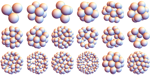
With simple permutation matrices, vertex sets for all 5 Platonic solids and 13 Archimedean solids with unit edges can be constructed:
In[]:=
icosahedron=[{0,1,"ϕ"},"Cyclic"]
Out[]=
{{-1,-ϕ,0},{-1,ϕ,0},{0,-1,-ϕ},{0,-1,ϕ},{0,1,-ϕ},{0,1,ϕ},{1,-ϕ,0},{1,ϕ,0},{-ϕ,0,-1},{-ϕ,0,1},{ϕ,0,-1},{ϕ,0,1}}
In[]:=
ϕ=1+;ξ=;tetrahedron=Select[{1,1,1}],EvenQ[Count[Sign[#],-1]]&Sqrt[8];cube=[{1,1,1}/2];octahedron=[{0,0,1}]Sqrt[2];icosahedron=[{0,1,ϕ},"Cyclic"]2;dodecahedron=Join@@[#,"Cyclic"]&/@{{1,1,1},{0,ϕ,1/ϕ}}(2/ϕ);cuboctahedron=[{0,1,1}]Sqrt[2];icosidodecahedron=Join@@[#,"Even"]&/@{0,0,ϕ},{1,ϕ,}2;rhombicuboctahedron=[{1,1,1+Sqrt[2]},"Even"]2;rhombicosidodecahedron=Join@@[#,"Even"]&/@{{1,1,},{,ϕ,2ϕ},{2+ϕ,0,}}2;truncatedcube=[{Sqrt[2]-1,1,1}](Sqrt[2]-1)2;truncatedoctahedron=[{0,1,2}]Sqrt[2];truncatedtetrahedron=Select[{1,1,3}],EvenQ[Count[Sign[#],-1]]&Sqrt[8];truncatedcuboctahedron=[{1,1+Sqrt[2],1+2Sqrt[2]}]2;truncateddodecahedron=Join@@[#,"Even"]&/@{{0,1/ϕ,2+ϕ},{1/ϕ,ϕ,2ϕ},{ϕ,2,ϕ+1}}(2ϕ-2);truncatedicosahedron=Join@@[#,"Even"]&/@{{0,1,3ϕ},{1,2+ϕ,2ϕ},{ϕ,2,2ϕ+1}}2;truncatedicosidodecahedron=Join@@[#,"Even"]&/@{1/ϕ,1/ϕ,3+ϕ},{2/ϕ,ϕ,1+2ϕ},1ϕ,,3ϕ-1,{2ϕ-1,2,2+ϕ},{ϕ,3,2ϕ}(2ϕ-2);snubcube=JoinSelect[{1,1/t,t},"Even"],EvenQ[Count[Sign[#],1]]&,Select[{1,1/t,t},"Odd"],OddQ[Count[Sign[#],1]]&Sqrt[2+4t-2t^2];snubdodecahedron=JoinSelectJoin@@[#,"Even"]&/@,OddQ[Count[Sign[#],-1]]&,SelectJoin@@[#,"Even"]&/@,EvenQ[Count[Sign[#],-1]]&2;poly={tetrahedron,cube,octahedron,icosahedron,dodecahedron,cuboctahedron,icosidodecahedron,rhombicuboctahedron,rhombicosidodecahedron,truncatedcube,truncatedoctahedron,truncatedtetrahedron,truncatedcuboctahedron,truncateddodecahedron,truncatedicosahedron,truncatedicosidodecahedron,snubcube,snubdodecahedron};
1
2
5
;t=2
ϕ
3
ϕ
2
ϕ
2
ϕ
2
ϕ
In[]:=
Grid[Partition[Graphics3D[Sphere[#,1/2],ImageSize->Tiny,Boxed->False]&/@poly,6]]
Rotating a Hypercube
Rotating a Hypercube
by: Enrique Zeleny
Rotate a hypercube around any axis in four dimensions, where there are six degrees of freedom; the associated matrices correspond to the special orthogonal group of order 4, SO(4).
Out[]=

What are Icosians?
What are Icosians?
It’s a set of 120 unit quaternions on . Start with (2,0,0,0) and (1,1,1,1), then apply plus/minus, permutations, halving and dot products with to get the 24-cell or octaplex. Add (0,1, 1/φ, φ) for the icosians , tetraplex, 600-cell or 120-cell centers.
-1====ijk
2
i
2
j
2
k
(1,i,j,k)
In[]:=
quads={{2,0,0,0},{1,1,1,1},{0,1,1/ϕ,ϕ}}/2/.ϕ->(1+Sqrt[5])/2;cell120=Flatten[ResourceFunction["SignedPermutations"][#,"Even"]&/@quads,1];cell24=Take[cell120,24]
Out[]=
{-1,0,0,0},{0,-1,0,0},{0,0,-1,0},{0,0,0,-1},{0,0,0,1},{0,0,1,0},{0,1,0,0},{1,0,0,0},-,-,-,-,-,-,-,,-,-,,-,-,-,,,-,,-,-,-,,-,,-,,,-,-,,,,,-,-,-,,-,-,,,-,,-,,-,,,,,-,-,,,-,,,,,-,,,,
1
2
1
2
1
2
1
2
1
2
1
2
1
2
1
2
1
2
1
2
1
2
1
2
1
2
1
2
1
2
1
2
1
2
1
2
1
2
1
2
1
2
1
2
1
2
1
2
1
2
1
2
1
2
1
2
1
2
1
2
1
2
1
2
1
2
1
2
1
2
1
2
1
2
1
2
1
2
1
2
1
2
1
2
1
2
1
2
1
2
1
2
1
2
1
2
1
2
1
2
1
2
1
2
1
2
1
2
1
2
1
2
1
2
1
2
1
2
1
2
1
2
1
2
1
2
1
2
In[]:=
icosians=SortBy[ResourceFunction["Quaternion"]@@#&/@cell120,Sort[{#,Conjugate[#]}]&];
In[]:=
RandomSample[icosians,5]
Out[]=
,,,,
Hexakis Triacontahedron
Hexakis Triacontahedron
The icosian quaternions ultimately function like rotation matrices:
tri=ResourceFunction["Quaternion"]@@#&/@{{0,1/ϕ,0,ϕ},{0,0,1,ϕ},{0,0,0,5ϕ/(ϕ+3)}}/.ϕ->(1+Sqrt[5])/2;all=Table[RootReduce[If[OddQ[g],1,-1]Table[#[[k]],{k,2,4}]]&/@Simplify[((icosians[[g]]**tri)**Conjugate[icosians[[g]]])],{g,1,120}];Graphics3D[{Polygon[#]&/@all},SphericalRegion->True,Boxed->False]
Out[]=

Vector Addition is Commutative
Vector Addition is Commutative
by: Izidor Hafner
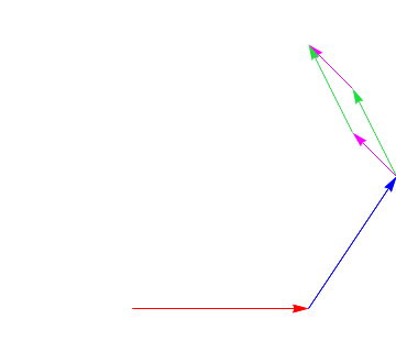
The Demonstration shows the commutativity of vector addition.
Out[]=
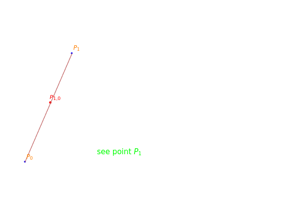
Vector Projection
Vector Projection
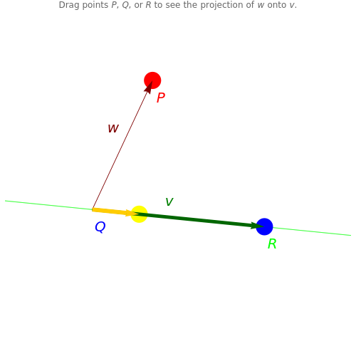
The yellow vector is the projection of the vector onto the vector .
QP
QR
Out[]=
Graphical Construction of a 2x2 Matrix and Its Inverse
Graphical Construction of a 2x2 Matrix and Its Inverse
by: Jodie Hoh
This Demonstration shows a pictorial representation of the relationship between a 2×2 matrix and its inverse. Drag the locators to determine two points; these define two vectors from the origin. The matrix has those vectors as its rows; it is shown on the lower left.
A
The inverse matrix is then shown on the lower right. The columns of the inverse matrix can be constructed from the two dashed vectors. The blue row of is orthogonal to the blue column of and the red row of is orthogonal to the red column of .
-1
A
A
-1
A
A
-1
A
Out[]=

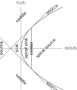
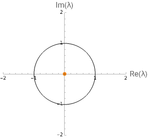
Eigenvalues and the Trace-Determinant Plane of a Linear Map
Eigenvalues and the Trace-Determinant Plane of a Linear Map
by: George Shillcock
Drag the point on the trace-determinant plane [1], and the corresponding eigenvalues are displayed around the unit circle in the complex plane.
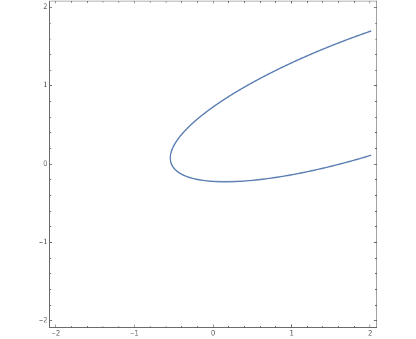
The graphic on the left shows the discriminant parabola and the lines for unit eigenvalues. Where in the trace-determinant plane are the eigenvalues the same? Can you make both eigenvalues have modulus one?
Let be a matrix; then the trace is the sum of the eigenvalues and the determinant is the product of the eigenvalues. The inverse relation is found by using the quadratic formula on the characteristic polynomial.
The eigenvalues of the matrix determine how the orbit/flow behaves. Can you find the critical point at which a period-doubling bifurcation occurs in the map/flow?
The graphic on the left shows the discriminant parabola and the lines for unit eigenvalues. Where in the trace-determinant plane are the eigenvalues the same? Can you make both eigenvalues have modulus one?
Let
A
22
tr(A)
det(A)
The eigenvalues of the matrix
A
In[]:=
Clear[tr]
Out[]=
Tetrahedron Volume
Tetrahedron Volume
The volume of a tetrahedron is equal to the determinant formed by writing the coordinates of the vertices as columns and then appending a row of ones along the bottom.
Out[]=

Circumsphere
Circumsphere
Finding a circumsphere has a simple matrix:
In[]:=
pts=RandomInteger[{0,9},{4,3}];mat={#.#,#[[1]],#[[2]],#[[3]],1}&/@Prepend[pts,{x,y,z}];MatrixForm[mat]
Out[]//MatrixForm=
2 x 2 y 2 z | x | y | z | 1 |
98 | 8 | 3 | 5 | 1 |
91 | 1 | 9 | 3 | 1 |
27 | 1 | 1 | 5 | 1 |
75 | 7 | 5 | 1 | 1 |
In[]:=
Show[{Graphics3D[Sphere[#,1]&/@pts],ContourPlot3D[Det[mat]==0,{x,-9,9},{y,-9,9},{z,-9,9}]}]
Out[]=

Five Point Conic
Five Point Conic
Five points determine a conic section. In this Demonstration, move up to six points, and see all the conic sections that pass through any subset of five points.
=0.
2 x | xy | 2 y | x | y | 1 |
2 x 1 | x 1 y 1 | 2 y 1 | x 1 | y 1 | 1 |
2 x 2 | x 2 y 2 | 2 y 2 | x 2 | y 2 | 1 |
2 x 3 | x 3 y 3 | 2 y 3 | x 3 | y 3 | 1 |
2 x 4 | x 4 y 4 | 2 y 4 | x 4 | y 4 | 1 |
2 x 5 | x 5 y 5 | 2 y 5 | x 5 | y 5 | 1 |
In[]:=
makeRow[{x_,y_}]:={,xy,,x,y,1};
2
x
2
y
In[]:=
Conic[x_,y_][pts_]:=Det[makeRow/@Join[{{x,y}},pts]];
Out[]=
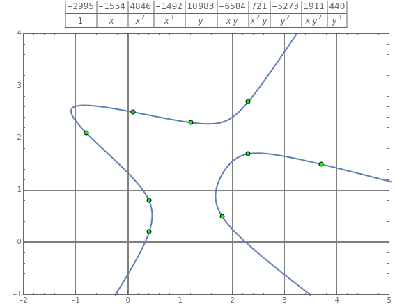
Nine-Point Cubic
Nine-Point Cubic
This Demonstration plots a cubic equation of the form +x+++y+xy+y++x+=0 in the Cartesian plane to pass through any nine points , . These cubic equations are often called elliptic curves. In this Demonstration, drag the points to see some of the many possible behaviors for a cubic equation.The coefficient values are rounded in the header, and should not be trusted when all values are low or zero. For some degenerate point configurations, such as the points marking the vertices and two points per side of a triangle, the matrix method used here may not work. A full method would employ special processing for degenerate lines and conics.
a
0
a
1
a
2
2
x
a
3
3
x
a
4
a
5
a
6
2
x
a
7
2
y
a
8
2
y
a
9
3
y
(,)
x
i
y
i
i=1,…,9
1 | x | 2 x | 3 x | y | xy | 2 x | 2 y | x 2 y | 3 y |
1 | x 1 | 2 x 1 | 3 x 1 | y 1 | x 1 y 1 | 2 x 1 y 1 | 2 y 1 | x 1 2 y 1 | 3 y 1 |
1 | x 2 | 2 x 2 | 3 x 2 | y 2 | x 2 y 2 | 2 x 2 y 2 | 2 y 2 | x 2 2 y 2 | 3 y 2 |
1 | x 3 | 2 x 3 | 3 x 3 | y 3 | x 3 y 3 | 2 x 3 y 3 | 2 y 3 | x 3 2 y 3 | 3 y 3 |
1 | x 4 | 2 x 4 | 3 x 4 | y 4 | x 4 y 4 | 2 x 4 y 4 | 2 y 4 | x 4 2 y 4 | 3 y 4 |
1 | x 5 | 2 x 5 | 3 x 5 | y 5 | x 5 y 5 | 2 x 5 y 5 | 2 y 5 | x 5 2 y 5 | 3 y 5 |
1 | x 6 | 2 x 6 | 3 x 6 | y 6 | x 6 y 6 | 2 x 6 y 6 | 2 y 6 | x 6 2 y 6 | 3 y 6 |
1 | x 7 | 2 x 7 | 3 x 7 | y 7 | x 7 y 7 | 2 x 7 y 7 | 2 y 7 | x 7 2 y 7 | 3 y 7 |
1 | x 8 | 2 x 8 | 3 x 8 | y 8 | x 8 y 8 | 2 x 8 y 8 | 2 y 8 | x 8 2 y 8 | 3 y 8 |
1 | x 9 | 2 x 9 | 3 x 9 | y 9 | x 9 y 9 | 2 x 9 y 9 | 2 y 9 | x 9 2 y 9 | 3 y 9 |
Out[]=
Adjacency Matrices of Manipulable Graphs
Adjacency Matrices of Manipulable Graphs
The adjacency matrix of a graph shows how the vertices are connected; when the entry at row , column is 1 in the matrix, the vertices and are connected. Moving the points leaves the adjacency matrix the same.
i
j
i
j
Out[]=

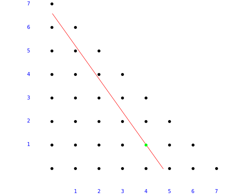
Sylvester’s Postage Stamp Problem
Sylvester’s Postage Stamp Problem
by: Izidor Hafner
J. J. Sylvester (1814–1897) posed the problem of finding the largest number that cannot be made up of some combination of 5p and 17p stamps.
In[]:=
FrobeniusNumber[{5,17}]
Out[]=
63
What is the greatest positive integer such that the Diophantine equation has no solution in non-negative integers? If and are relatively prime numbers, the equation has a solution in integers for any integer and has a solution in non-negative integers for any integer greater than .
c
ax+by=c
a
b
c
c
ab-2
Out[]=
Tensor Equation of a Plane
Tensor Equation of a Plane
by: Brad Klee
The general equation of a plane can be written as , where coefficients , , , and are determined using a set of matrices. The simplification of the plane equations to one tensor equation proceeds from the similarity of the three-vector equations for , , , and . These equations can be rewritten together using the antisymmetric permutation tensor ; however, the three-vectors , , for points in and the origin need to be rewritten as four-vectors so that they have a compatible dimension. The first three components of the vectors , , , and are equal to the coordinates of a point in and the fourth component of these vectors is . Similarly, the first three components of the vector are equal to the free variables , , and , while the fourth component of this vector is . The matrix allows the first, second, and third components of a four-vector to be selected for summation. Choosing three distinguishable points, the equation for a plane can be written in tensor notation as =0. A point-to-plane distance function can also be written in tensor notation. The distance between an origin and a plane can be written as: . Tensor notation for planes and distances could be very useful to material scientists who would like to define coordinate systems and compute distance functions without using Miller indices.
A+B+C+D=0
q
1
q
2
q
3
A
B
C
D
A
B
C
D
ijkl
ϵ
q
1
q
2
q
3
3
O
q'
i
q''
j
q'''
k
O
l
3
1
e
q
1
q
2
q
3
1
η
lq
ijkl
ϵ
q'
i
q''
j
q'''
k
e
l
λ
O
P
λ(O,P)=
ijkl
ϵ
q'
i
q''
j
q'''
k
O
l
-1
ijkl
ϵ
q'
i
q''
j
q'''
k
η
lq
mnpq
ϵ
q'
m
q''
n
q'''
p
Out[]=

Brillhart’s Cubic and e^(Sqrt[163] π)
Brillhart’s Cubic and e^(Sqrt[163] π)
The Brillhart matrix has eigenvalues that give the solutions of b^3-8 b-10=0. In 1965, Brillhart noticed this led to an exotic continued fraction, with numerous large terms early in the expansion.
In[]:=
MatrixForm[{{0,2,2},{1,0,2},{2,1,0}}]
Out[]//MatrixForm=
0 | 2 | 2 |
1 | 0 | 2 |
2 | 1 | 0 |
In[]:=
bc=Eigenvalues[{{0,2,2},{1,0,2},{2,1,0}}][[1]]ContinuedFraction[N[bc,240]]
Out[]=
Out[]=
{3,3,7,4,2,30,1,8,3,1,1,1,9,2,2,1,3,22986,2,1,32,8,2,1,8,55,1,5,2,28,1,5,1,1501790,1,2,1,7,6,1,1,5,2,1,6,2,2,1,2,1,1,3,1,3,1,2,4,3,1,35657,1,17,2,15,1,1,2,1,1,5,3,2,1,1,7,2,1,7,1,3,25,49405,1,1,3,1,1,4,1,2,15,1,2,83,1,162,2,1,1,1,2,2,1,53460,1,6,4,3,4,13,5,15,6,1,4,1,4,1,1,2,1,16467250,1,3,1,7,2,6,1,95,20,1,2,1,6,1,1,8,1,48120,1,2,17,2,1,2,1,4,2,3,1,2,23,3,2,1,1,1,2,1,27,325927,1,60,1}
Due to the oddities of modular forms, and -24 are very close to each other and +744.
π
163
e
24
(2+bc)
3
640320
Column[{AccountingForm[N[E^(Sqrt[163]π),32]],AccountingForm[N[(2+bc)^24-24,32]],AccountingForm[N[640320^3+744,32]]}]
Out[]=
262537412640768743.99999999999925 |
262537412640768743.99999999999925 |
262537412640768744.00000000000000 |
Extraordinary Lines -- How to do it Fast.
Extraordinary Lines -- How to do it Fast.
From a set of points, find all lines of three or more points.
In[]:=
pts={{0,0},{6,-6},{-6,6},{-2,-6},{2,6},{6,6},{-6,-6},{-6,0},{6,0},{0,3},{0,-3}};lines=ResourceFunction["FindExtraordinaryLines"][pts]
Out[]=
{{1,2,3},{1,4,5},{1,6,7},{1,8,9},{1,10,11},{2,4,7},{2,6,9},{2,8,11},{3,5,6},{3,7,8},{3,9,10},{4,6,11},{5,7,10},{6,8,10},{7,9,11}}
What’s the fastest way to calculate a lot of lines?
In[]:=
Graphics[{Green,Line[pts[[#]]]&/@lines,Black,Table[Style[Text[n,pts[[n]]],20],{n,1,Length[pts]}]}]
Out[]=
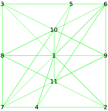
Here’s the code I used. RowReduce seems to be the fastest way to calculate lines.
FindExtraordinaryLines[pts_?MatrixQ]:=SortBy[Select[(Union[Flatten[#1,1]]&)/@GatherBy[Subsets[Range[Length[pts]],{2}],RootReduce[RowReduce[ArrayPad[pts[[#1]],{{0,0},{0,1}},1]]]&],Length[#1]>2&],-Length[#1]&];
In[]:=
ArrayPad[{{6,0},{0,3}},{{0,0},{0,1}},1]
Out[]=
{{6,0,1},{0,3,1}}
Some Special Types of Matrices
Some Special Types of Matrices
A matrix is if it has rows and columns. If there is only one row or column, the matrix can be treated like a vector.For a square matrix, the number of rows equals the number of columns.A zero matrix acts like the number zero for matrices of the same dimensions. The main diagonal of a square matrix runs from the top-left corner to the bottom-left corner.The identity matrix is square, with ones on the main diagonal and zeros elsewhere. It acts like the number one for matrix multiplication. A diagonal matrix is a square matrix that has zeros off the main diagonal. Let be and , where and .The transpose of the matrix , written , reverses the rows and columns of , so that is and . Another way to think of is as the reflection of in its main diagonal.Let be an square matrix and , where .A square matrix is symmetric if , so that =.A square matrix is skew-symmetric if , so that =-. A skew-symmetric matrix is therefore zero on the main diagonal.A square matrix is upper triangular if it is zero below the main diagonal. A square matrix is lower triangular if it is zero above the main diagonal.
A
m×n
m
n
A
m×n
A=()
a
ij
1≤i≤m
1≤j≤n
A
A
A
A
n×m
A=()
a
ji
A
A
B
n×n
B=
b
ij
1≤i,j≤n
B
B=B
b
ij
b
ji
B
B=-B
b
ij
b
ji
B
B
Out[]=
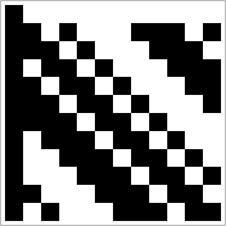
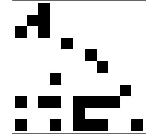
Small Hadamard Matrices
Small Hadamard Matrices
A Hadamard matrix is a square matrix with all entries equal to or , with its rows mutually orthogonal. Half of the corresponding pairs of entries in any two rows have the same sign and half have the opposite sign.
+1
-1
It is conjectured that a Hadamard matrix of order exists for all integers divisible by 4. However, many orders are unsolved, including 668, 716 and 892.
n
In[]:=
hadamard=;Manipulate[ArrayPlot[1+hadamard[[k/4]],ImageSize{450,450}],{{k,12,"order"},4,108,4,Appearance"Labeled"},SaveDefinitionsTrue]
Out[]=
In[]:=
hadamard[[16,4]].hadamard[[16,5]]
Out[]=
0
The Space of Inner Products
The Space of Inner Products
This Demonstration shows the space of triples with , which can be identified with the positive definite quadratic form , together with the orbits of the natural action of the special linear group of matrices with determinant 1. You can vary the quadratic form by changing its three parameters (, , and the discriminant ) and see the point corresponding to the form move within the region of space where the positive definite quadratic forms lie. By varying the matrix parameters you can see the image of the fixed form (which corresponds to another quadratic form with the same discriminant). You also see the part of the orbit of the action contained within the displayed area by checking the “show orbit” checkbox.
(a,b,c)
ab>
2
c
a+cxy+b
2
x
2
y
SL(2,)
2×2
a
b
δ=ab-
2
c
A positive definite quadratic form (or, equivalently, an inner product) on can be identified with a matrix , where . The bilinear form is then
·
.
=
. An invertible matrix acts on via the formula ·A·S, which corresponds to another positive definite quadratic form. If has determinant 1 (i.e. belongs to ), the form has the same discriminant (determinant of the corresponding matrix). Thus the orbits of the action consist of forms with the same value of the discriminant.
2
2×2
A
a | c |
c | b |
ab>
2
c
(x | y) |
a | c |
c | b |
x |
y |
a 2 x 2 y |
S
A
T
S
S
SL(2,)
Out[]=

Creating Self-Similar Fractals with Hutchinson Operators
Creating Self-Similar Fractals with Hutchinson Operators
by: Garrett Nelson
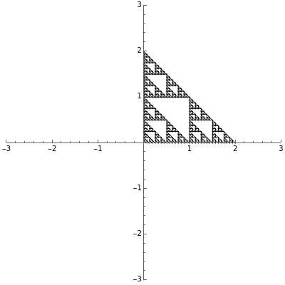
A map is a contraction mapping if for all points , , , where . A similitude is a contraction mapping that is a composition of dilations, rotations, translations, and reflections. A two-dimensional Hutchinson operator maps a plane figure to the union of its images under a finite collection of similitudes. The orbit of a plane figure under such an operator can form a self-similar fractal. In this Demonstration you can vary three similitudes (without reflection) to see what self-similar fractals are possible.
As long as the initial subset of the plane is compact, iterations of the Hutchinson operator converge to the same fractal, yet the convergence is faster for some subsets than others; in particular, the set of the three fixed points of the three similitudes gives fast convergence.
To better see what a Hutchinson operator does, use “constant points” to start with the same three points rather than.
M
x
y
|M(x)-M(y)|≤r|x-y|
0≤r<1
As long as the initial subset of the plane is compact, iterations of the Hutchinson operator converge to the same fractal, yet the convergence is faster for some subsets than others; in particular, the set
F
To better see what a Hutchinson operator does, use “constant points” to start with the same three points rather than
F
Out[]=
The Boundary of Periodic Iterated Function Systems
The Boundary of Periodic Iterated Function Systems
by: Jarek Duda
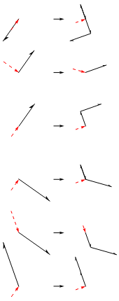
This Demonstration shows approximations of the boundary (clockwise) of some discrete families of iterated functional systems (IFS), =(F+i), which can be thought of as the fractional part of numeration systems with a complex base, .
F
z
n-1
⋃
i=0
z=D/2+i
n-
2
(D/2)
Change and to choose one of the periodic cases. The next slider “shown recurrence level” lets you choose the level of approximation and the rotation of the recurrence relation; for example, ‘’ represents the iteration. These relations show that an edge with given previous direction (red) changes into the resulting sequence of edges. Ignoring order gives the matrix with dominant eigenvalue () and corresponding eigenvector, which gives the limit distribution of the number of edges. In the limit the figure becomes a fractal with the Hausdorff dimension .
n
D
1
12
λ
2λ
log
n
Out[]=

Rauzy Fractals of Order Four
Rauzy Fractals of Order Four
by: Dieter Steemann
Experiment with 3D tilings based on unimodular Pisot substitutions of order four.
The common Rauzy fractal set is associated with the tribonacci substitution. Here the generation method based on a unimodular substitution of the Pisot type of order three (as demonstrated in [1]) is expanded to “tetrabonacci” substitutions of order four. An introduction to Pisot substitutions and Rauzy fractals is given by Arnoux and Ito [2]. Pisot means that the substitution has an incidence matrix with a unique eigenvalue of modulus greater than 1, and all other eigenvalues of modulus less than 1. Unimodular refers to a matrix with a determinant of .
±1
The core algorithms of this program follow the work of Barge and Kwapisz [3] expanded to order four. The tilings are defined by substitution rules using an alphabet of four letters, in this case. The generated output is a 4D surface, where each letter of the substitution result corresponds to a specific 4D face. These faces are projected into the 3D space using the corresponding eigenvector of the Pisot eigenvalue. In the 3D space, every 4D face corresponds to a 3D prototile. This can be experienced by changing the 3D viewpoint or by manual rotation of the image result, best at low iteration levels and with colored edges. The given rules originate from our own experiments; they are different, but may include symmetries.
{1,2,3,4}
Out[]=

Phase Portraits, Eigenvectors, and Eigenvalues
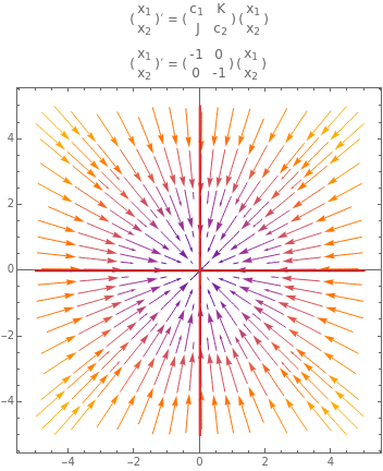
Phase Portraits, Eigenvectors, and Eigenvalues
This Demonstration plots an extended phase portrait for a system of two first-order homogeneous coupled equations and shows the eigenvalues and eigenvectors for the resulting system. You can vary any of the variables in the matrix to generate the solutions for stable and unstable systems. The eigenvectors are displayed both graphically and numerically. The following phenomena can be seen: stable and unstable saddle points, lines of equilibria, nodes, improper nodes, spiral points, sinks, nodal sinks, spiral sinks, saddles, sources, spiral sources, nodal sources, and centers.
Out[]=


Sporadic Groups
Sporadic Groups
A group is a set of elements that is closed under an associative binary operation such that contains an identity element and each element in has an inverse .For example, consider a cube. You can rotate it in several different ways to produce an indistinguishable copy of the original; such an operation is called a symmetry. Doing two successive rotations is equivalent to doing some single rotation. In all, a cube has 24 rotational symmetry elements (not counting an equal number that involve reflections).A tetrahedron has 12 rotational symmetry operations, which constitute a subgroup of the symmetries of the cube.A normal subgroup of a group is defined by the property that for . (For some intuition about normal subgroups, see [2].) For example, is a normal subgroup of .A group is simple if it has no normal subgroups apart from the trivial ones and itself. A simple group is like a prime number in arithmetic. Groups can be analyzed by repeatedly factoring out the largest normal subgroups.There are 18 infinite families of finite simple groups plus 26 exceptional sporadic groups. This Demonstration provides binary generator matrices and for 23 of the 26 sporadic groups (the remaining three are too large). From these, a binary number can select a multiplication sequence of these generators.An enormously complex proof of the theorem classifying all finite simple groups was tentatively completed by Daniel Gorenstein in 1983.
G
G
e
g
G
-1
g
T
C
N
G
gN=N
-1
g
g∈G
T
C
G
{e}
G
a
b
Out[]=
The generators of a group are a set of elements such that every element of the group can be expressed as a product of a finite number of generators. For example, this Demonstration has 10×10 matrices and over as generators for the 7920 elements of the Mathieu group . (The binary operation is matrix multiplication, and is the Galois field with two elements, 0 and 1.) For element 7920, the decimal sequence for the product is 85283493; the equivalent binary number is 101000101010101001010100101. Substituting for 1 and for 0 gives the product .The 23 sporadic groups in this Demonstration are:
a
b
GF(2)
M
11
GF(2)
a
b
ababbbabababababbabababbaba
Name | Generatorsize | Grouporder | |
M11 | Mathieugroup M 11 | 10×10overGF(2) | 7920 |
M12 | Mathieugroup M 12 | 10×10overGF(2) | 95040 |
M22 | Mathieugroup M 22 | 10×10overGF(2) | 443520 |
M23 | Mathieugroup M 23 | 11×11overGF(2) | 10200960 |
M24 | Mathieugroup M 24 | 11×11overGF(2) | 244823040 |
J1 | Jankogroup J 1 | 20×20overGF(2) | 175560 |
HS | Higman–Simsgroup | 20×20overGF(2) | 44352000 |
McL | McLaughlingroup | 22×22overGF(2) | 898128000 |
Co2 | Conwaygroup Co 2 | 22×22overGF(2) | 42305421312000 |
Co3 | Conwaygroup Co 3 | 22×22overGF(2) | 495766656000 |
Co1 | Conwaygroup Co 1 | 24×24overGF(2) | 4157776806543360000 |
Ru | RudvalisGroup | 28×28overGF(2) | 145926144000 |
HJ | Hall–Jankogroup | 36×36overGF(2) | 604800 |
He | Heldgroup | 51×51overGF(2) | 4030387200 |
F22 | Fischergroup F 22 | 78×78overGF(2) | 64561751654400 |
J3 | Jankogroup J 3 | 80×80overGF(2) | 50232960 |
J4 | Jankogroup J 4 | 112×112overGF(2) | 86775571046077562880 |
Suz | Suzukigroup | 142×142overGF(2) | 448345497600 |
Th | Thompsongroup | 248×248overGF(2) | 90745943887872000 |
ON | ONangroup | 154×154overGF(3) | 460815505920 |
F23 | Fischergroup F 23 | 253×253overGF(3) | 4089470473293004800 |
Ly | Lyonsgroup | 111×111overGF(5) | 51765179004000000 |
HN | Harada–Nortongroup | 133×133overGF(5) | 273030912000000 |
These three sporadic groups were judged to be too large for this Demonstration:
Name | Generatorsize | Grouporder | |
F24 | Fischergroup F 24 | 781×781overGF(3) | 1255205709190661721292800 |
B | BabyMonster | 4370×4370overGF(2) | 4154781481226426191177580544000000 |
M | Monster | 196882×196882overGF(2) | 808017424794512875886459904961710757005754368000000000 |
Matrices, Vectors and Structured Data do a Lot!
Matrices, Vectors and Structured Data do a Lot!
Virtually all computer application rely on matrices. Matrices are fast. All large computer models, from weather to space exploration to special effects, use matrices heavily. New applications in AI rely on data carefully stored as matrices. Most mathematical problems can be converted to linear algebra problems. Structured data is everywhere.
In[]:=
PolyhedronData["Tetrahedron"]
Out[]=

CITE THIS NOTEBOOK
CITE THIS NOTEBOOK
Mathematical Games: Linear Algebra magic
by Ed Pegg
Wolfram Community, STAFF PICKS, June 20, 2024
https://community.wolfram.com/groups/-/m/t/3197300
by Ed Pegg
Wolfram Community, STAFF PICKS, June 20, 2024
https://community.wolfram.com/groups/-/m/t/3197300