=2.718...
n
Problem from classical probability
Problem from classical probability
(Crux Mathematicorum, 2024, Vol. 50, No. 4) You play a game by repeatedly rolling an n-sided fair die until for the first time you get a number that is less than or equal to a previously rolled number, at which point in time the game ends. On average, how many times do you roll before the game ends? What happens as gets unboundedly large?
n
Simulation
Simulation
Lets do some experiments. Say you have a fair dice with 6 faces.For instance, if in the first roll you have 2 and in the second roll we have 3, we can roll the dice for the third time. If the second roll shows 1, the process halts.
Notice that the maximum number of rolling for a 6-face dice is 7 because if we have {6,5,4,3,2,1} in 6 steps, the game stops at the 7th roll regardless of what we have. Thus for a -face dice, each run terminates at most rolls.
n
n+1
Lets run 20000 rounds of the dice experiment for any given -face dice. In each round, we record the face value of the dice after each roll using stack data structure because it is fast to add element to this mutable object and the peek operation is convenient for retrieving the value from the previous step:
n
stk=CreateDataStructure["Stack"];
roll[n_Integer]:=Table[rollNextQ=True;stk["DropAll"];stk["Push",RandomInteger[{1,n}]](*atleastrollonce*);While[rollNextQ,curr=RandomInteger[{1,n}];If[curr<=stk["Peek"],rollNextQ=False];stk["Push",curr];];stk["Elements"],{i,20000}]
For 6-face dice, we run simulation:
In[]:=
experiments=roll[6];Short[experiments]
Out[]//Short=
{{5,3},{2,5,1},{5,1},{6,6},19992,{4,6,6},{4,3},{4,1},{5,1}}
Visualize the dice face for some samples:
In[]:=
TableForm[Row/@Map[sixfaces,RandomSample[experiments,8],{2}],TableHeadings{"Sample "<>ToString[#]&/@Range[8],None}]
Out[]//TableForm=
Sample 1 | |
Sample 2 | |
Sample 3 | |
Sample 4 | |
Sample 5 | |
Sample 6 | |
Sample 7 | |
Sample 8 |
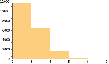
The distribution of the length of each run and the average is
In[]:=
With[{lenList=Length/@experiments},{Histogram[lenList],N@Mean[lenList]}]
Out[]=
,2.5217
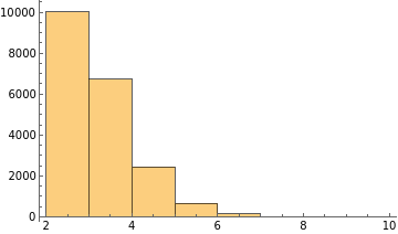
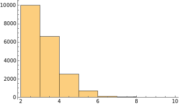
If we repeat the same process for 500-face, 5000-face and 50000-face dices, the results look like below:
In[]:=
TableForm[With[{lenList=Length/@#},{Histogram[lenList],N@Mean[lenList]}]&/@{roll[500],roll[5000],roll[50000]},TableHeadings->{{"500 faces","5000 faces","50000 faces"},{"Distribution","Avg. length of run"}},TableAlignments->Center]
Out[]//TableForm=
Distribution | Avg. length of run | |
500 faces | 2.7101 | |
5000 faces | 2.7189 | |
50000 faces | 2.7235 |
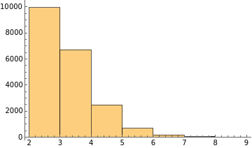
The averages are not very far from 2.72. Actually the theoretical limit is indeed as the number of faces of a dice approaches infinity.
=2.718...
In[]:=
N@
Out[]=
2.71828
Proof
Proof
There are two ways. One is more rigorous and the other is an educated guess plus some calculus.
1. Say we have a 6-face dice and we want to find the expectation value of the size of runs (X). By definition the expectation is weighted sum of each occurrence:
E=1·P(X=1)+2·P(X=2)+3·P(X=3)+4·P(X=4)+5·P(X=4)+6·P(X=6)+7·P(X=7)
We can convert this sum into two dimensional array and switch the order of sum (denoting =P(X=i)):
P
i
E
P 1 | P 2 | P 3 | P 4 | P 5 | P 6 | P 7 |
· | P 2 | P 3 | P 4 | P 5 | P 6 | P 7 |
· | · | P 3 | P 4 | P 5 | P 6 | P 7 |
· | · | · | P 4 | P 5 | P 6 | P 7 |
· | · | · | · | P 5 | P 6 | P 7 |
· | · | · | · | · | P 6 | P 7 |
· | · | · | · | · | · | P 7 |
Notice that i-th row sum is . Therefore the expectation value can be evaluated in a different manner:
P(X>=i)=P(X>i-1)
E
E=P(X>=1)+P(X>=2)+P(X>=3)+P(X>=4)+P(X>=5)+P(X>=6)+P(X>=7)
Lets think about the probability for at least 4 rolls in a run. This requires that the three numbers before the fourth roll is in ascending order. This is precisely “6 choose 3” and the probability of choosing each element in the three-item bucket is 1/6:
In[]:=
TraditionalForm[HoldForm[Binomial[6,3]*(1/6)^3]]
Out[]//TraditionalForm=
6 |
3 |
3
1
6
What about at least 5 rolls? This requires that the four distinct numbers before the fifth roll is in ascending order. This is precisely 6 choose 4 and the probability of choosing each element in the four-item bucket is 1/6:
In[]:=
TraditionalForm[HoldForm[Binomial[6,4]*(1/6)^4]]
Out[]//TraditionalForm=
6 |
4 |
4
1
6
Likewise we can apply the argument to other terms. In general, for 6-face dice is:
P(X>=k)
In[]:=
TraditionalForm[HoldForm[Binomial[6,k]*(1/6)^k]]
Out[]//TraditionalForm=
6 |
k |
k
1
6
Sum up all terms:
In[]:=
TraditionalForm[Inactivate[Sum[HoldForm[Binomial[6,k]*(1/6)^k],{k,0,6}],Sum]]
Out[]//TraditionalForm=
6
∑
k=0
6 |
k |
k
1
6
This is precisely the binomial expansion of
In[]:=
TraditionalForm[HoldForm[(1+1/6)^6]]
Out[]//TraditionalForm=
6
1+
1
6
From Our previous rolling 6-dice experiment, we have an average around . This is very close to the theoretic value:
2.5217
In[]:=
N@(1+1/6)^6
Out[]=
2.52163
Replace 6 with for and then take to infinity:
n
n
In[]:=
DiscreteLimit[(1+1/n)^n,n->Infinity]//Framed
Out[]=
2. If you have reached this part, the following argument should not be too ridiculous. For infinitely sided dice we have a series instead of finite sum:
E=P(X>=1)+P(X>=2)+P(X>=3)+P(X>=4)+P(X>=5)+P(X>=6)+P(X>=7)+...
Lets thinks about at least roll 4 times, . This requires that first 3 numbers are in ascending order. If the chance of picking any number is even, then the occurrence of orders of elements in the tuple must be even. Only one of the permutation is valid, which is of strict ascending order:
P(X>=4)
In[]:=
Permutations[{"Large","Median","Small"}]
Out[]=
{{Large,Median,Small},{Large,Small,Median},{Median,Large,Small},{Median,Small,Large},{Small,Large,Median},{Small,Median,Large}}
In[]:=
1/3!
Out[]=
1
6
Same argument applies to other cases. Therefore the expectation value is if you have seen it in Calculus-1 course:
In[]:=
Sum[1/n!,{n,0,Infinity}]//Framed
Out[]=
The limit for i-th term with also confirms with the argument above:
P(X>=i)
In[]:=
DiscreteLimit[Binomial[n,k]*(1/n)^k,n->Infinity]
Out[]=
1
kGamma[k]
In[]:=
FullSimplify[%,Assumptions->k∈PositiveIntegers]
Out[]=
1
k!
Comment
Comment
This experiment demonstrates a possible Monte-Carlo method to estimate but with slow convergence rate.
Utilities
Utilities
In[]:=
sixfaces=AssociationThread[{1,2,3,4,5,6}->Import/@{"https://i.sstatic.net/FdfMj.png","https://i.sstatic.net/Qv7w6.png","https://i.sstatic.net/WayOQ.png","https://i.sstatic.net/mgjkA.png","https://i.sstatic.net/qa5bK.png","https://i.sstatic.net/T8szh.png"}];
CITE THIS NOTEBOOK
CITE THIS NOTEBOOK
Make e=2.718... at home with rolling dice
by Shenghui Yang
Wolfram Community, STAFF PICKS, September 11, 2024
https://community.wolfram.com/groups/-/m/t/3271711
by Shenghui Yang
Wolfram Community, STAFF PICKS, September 11, 2024
https://community.wolfram.com/groups/-/m/t/3271711