Abstract: Rotational grazing has been a popular sustainable farming practice, which has been shown to increase yields and environmental health compared to continuous grazing.In this grazing system, land is divided into several paddocks, and the livestock is moved from one to another after some time, while empty paddocks are allowed to fallow. On the contrary, continuous grazing involves containing the animals in one singular fenced area. In this project, agent - based modeling was used in a computer simulation to show the dynamical change and interaction of the cows and the grass in different paddock situations and rotation periods over time.This simulation incorporates an explicit spatial structure, unlike previous models, and was created in NetLogo, a computer programming language that creates multi - agent environment and allows the user to interact with its interface.In this simulation, grass and cows were used as agents. Data was collected and analyzed from the resulting simulation.The health of the cows and the energy of the grass were used to quantitatively describe the productivity of the pasture. Several experiments were conducted to test different variables that would affect productivity by changing quantities on the NetLogo interface.The results from running the simulation show that the smallest herd of cows on a short rotation schedule will result in the most productive rotational grazing system.Nevertheless, the model proved that the most productive is a continuous grazing system. Further development of the simulation will be necessary to create more realistic conditions.
Background
Background
I created this project for my school science fair last year, and I decided to revisit the project for my AP Environmental Science class and to utilize my new Wolfram skills to produce better data and improve analysis and results. Rotational grazing is a farming practice that involves moving livestock between paddocks with a regular schedule. Using rotational grazing, a pasture is divided into multiple paddocks and only one or some paddocks is grazed at one time. It has been theorized that a management intensive grazing system, meaning increased paddock quantity as well as shorter grazing period results in the greatest yields. On the contrary, continuous grazing involves only one paddock, and the forage is not allowed to fallow. Previous research has been done using mathematical equations to model rotational grazing and its yields. Rotational grazing has been shown to provide for a larger amount of animals and result in higher yields of forage. Intensive rotational grazing can substantially increase long-term productivity in a pasture compared to other methods.
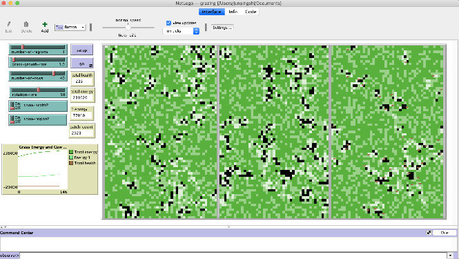
NetLogo provides a programmable environment for agent-based modeling. It can support multiple agents, that are stationary patches, mobile turtles, and the observer. Patches are lattice sites, specifically two-dimensional squares on a continuous plane. In most simulations, turtles move from patch-center to patch-center. Agents can interact with each other. For instance, the observer issues instructions for the patches and turtles, and the turtles can interact with the patches. Agent-based modeling is particularly useful in modeling change in complex systems over time. NetLogo also has an integrated user-interface, which allows one to create buttons, sliders, monitors, plots and other objects that allows the observer to watch and modify the setup.
My question in this experiment is “What conditions for rotational grazing are optimal for high yields of forage and livestock in a pasture?”
Simulation
Simulation
There are two types of agents in the habitat : the grass and the cows. The grass has four different lengths indicated by their color and the numbers 0,1,2,3. The set - up procedure initially sets all patches to the state 2 of grass with energy 20. Each cow is then also assigned to a health value, which is initially 0.
Four parameters can be entered in the program interface using sliders: the rotation time, number of cows, number of paddocks, and the rate of grass growth. Rotation time is measured in ticks and each tick is one day.
Update Algorithm for Grass Growth and Consumption: At each tick (time increasing by one), each patch chooses a random number between 1 and 100, and if this randomly chosen number is less than the given grass-growth-rate, the grass energy at this patch will increase to the next level and the color shown on that patch changes respectively. If the grass is already at the highest energy level, then it stays at that level.
Update Algorithm for Cow Movement and Rotation: All cows are in the same paddock during one rotation, and all other paddocks are free of cows. For each cow, its location updates every tick, and the cow can move to one of eight neighboring points. The cows are restricted from moving outside of their current region. After a rotation time, all the cows in the paddock move to the next paddock. Specific values for the gains and losses in cow health and grass energy from consumption and movement are given in the Table below.
Out[]=
| cow health | grass energy | ||||||||
eat grass |
| -10 | ||||||||
grass regrow | | 10 | ||||||||
cow move | -0.75 | |
Wolfram Analysis
Wolfram Analysis
I input the NetLogo file into Wolfram and performed analysis through my Wolfram Desktop application. Here, I run the simulation to test certain variables and record the data.
Start NetLogo and open project file
In[]:=
<<NetLogo`;NLStart["/Applications/NetLogo 6.1.0/"];NLLoadModel[ToFileName[{"Documents"},"grazing.nlogo"]]
Set constants
NLCommand["set grass-growth-rate",1.0];NLCommand["set number-of-cows",50];NLCommand["set rotation-time",20];
Define functions used for analysis
In[]:=
testnumregion[numregion_]:=Module[{},NLCommand["set number-of-regions",numregion,"setup"];data=NLDoReport["go","list(health-sum) (energy-sum)",200];{Map[#[[1]]/50&,data],Map[#[[2]]/10000&,data]}]
In[]:=
repeattest[numregion_]:=Table[testnumregion[numregion],10]
In[]:=
finalhealth[x_]:=Map[Last[#]&,Map[#[[1]]&,x]]
In[]:=
finalenergy[x_]:=Map[Last[#]&,Map[#[[2]]&,x]]
In[]:=
fullhealthdata[x_]:=Map[#[[1]]&,x]
In[]:=
fullenergydata[x_]:=Map[#[[2]]&,x]
In[]:=
meanall[x_]:=Map[Mean[#]&,x]
Experiment 1: Number of Paddocks
Experiment 1: Number of Paddocks
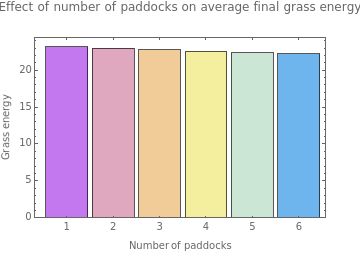
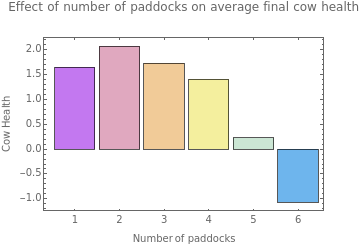
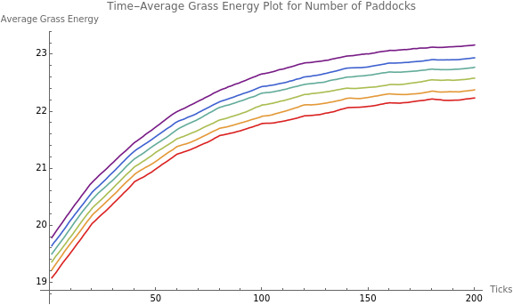
I tested the effect of the number of paddocks that the pasture is divided into (1-6). I used the average health of a cow and average energy of a patch as dependent variables. Each trial lasted 200 ticks and each variable was tested with 10 trials.
Generate data by testing each variable
In[]:=
paddock1=repeattest[1];paddock2=repeattest[2];paddock3=repeattest[3];paddock4=repeattest[4];paddock5=repeattest[5];paddock6=repeattest[6];
Clean the data and find the final values for health and energy
In[]:=
paddockdata={paddock1,paddock2,paddock3,paddock4,paddock5,paddock6};healthdata=Map[finalhealth[#]&,paddockdata];energydata=Map[finalenergy[#]&,paddockdata];paddockenergy=Map[Mean[#]&,energydata];paddockhealth=Map[Mean[#]&,healthdata];
Create table of results of final average health and energy
In[]:=
Column[{"Health",Grid[Prepend[(MapThread[Append,{MapThread[Prepend,{healthdata,Range[1,6]}],paddockhealth}]),Join[{"# of paddocks"},Range[1,10],{"average"}]],FrameAll],"Energy",Grid[Prepend[(MapThread[Append,{MapThread[Prepend,{energydata,Range[1,6]}],paddockenergy}]),Join[{"# of paddocks"},Range[1,10],{"average"}]],FrameAll]}]
Out[]=
Health | ||||||||||||||||||||||||||||||||||||||||||||||||||||||||||||||||||||||||||||||||||||
| ||||||||||||||||||||||||||||||||||||||||||||||||||||||||||||||||||||||||||||||||||||
Energy | ||||||||||||||||||||||||||||||||||||||||||||||||||||||||||||||||||||||||||||||||||||
|
Generate bar charts to compare average final health and energy
In[]:=
BarChart[paddockenergy,PlotLabel"Effect of number of paddocks on average final grass energy",ChartLabelsRange[1,6],ChartStyle"Pastel",FrameTrue,FrameLabel{{"Grass energy",""},{"Number of paddocks",""}}]
Out[]=
In[]:=
BarChart[paddockhealth,PlotLabel"Effect of number of paddocks on average final cow health",ChartLabelsRange[1,6],ChartStyle"Pastel",FrameTrue,FrameLabel{{"Cow Health",""},{"Number of paddocks",""}}]
Out[]=
Find the data to generate time series graphs
In[]:=
allhealth=Map[fullhealthdata[#]&,paddockdata];allenergy=Map[fullenergydata[#]&,paddockdata];
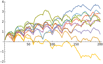
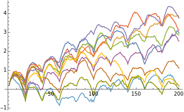
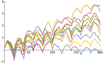
Create graphs to show each trial’s progression for each variable
In[]:=
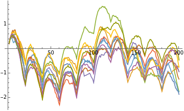
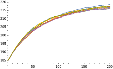
Map[ListLinePlot[#]&,allhealth]
Out[]=
,
,
,
,
,
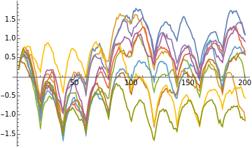
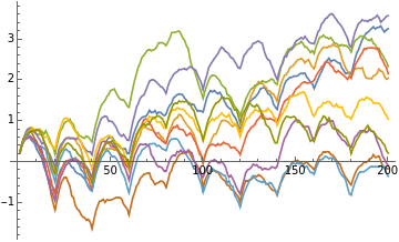
In[]:=
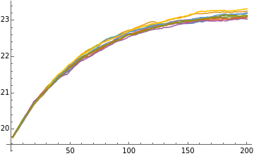
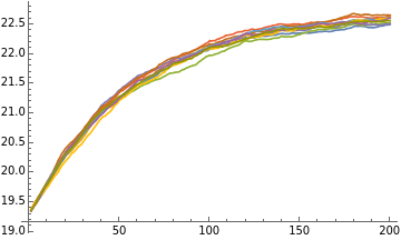
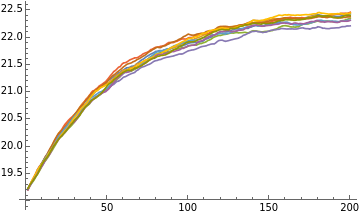
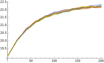
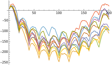
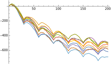
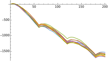
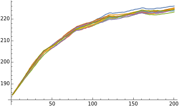
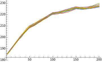
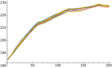
Map[ListLinePlot[#]&,allenergy]
Out[]=
,
,
,
,
,
Transpose all the trials together by tick
In[]:=
healthticks=Map[Transpose[#]&,allhealth];energyticks=Map[Transpose[#]&,allenergy];
In[]:=
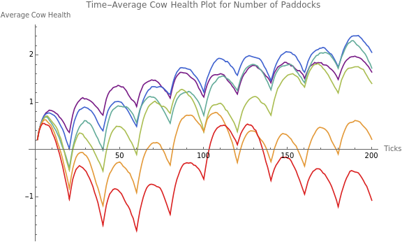
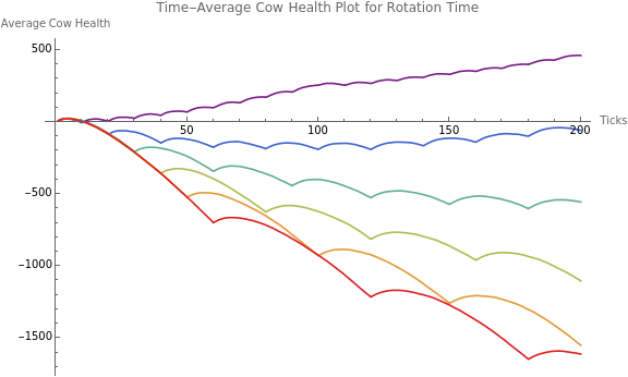
healthplot=ListLinePlot[Map[meanall[#]&,healthticks],AxesLabel{"Ticks","Average Cow Health"},PlotLegends{Range[1,6]},ImageSizeLarge,PlotStyle"Rainbow",PlotLabel"Time-Average Cow Health Plot for Number of Paddocks"]
Out[]=
In[]:=
energyplot=ListLinePlot[Map[meanall[#]&,energyticks],PlotRangeAll,AxesLabel{"Ticks","Average Grass Energy"},ImageSizeLarge,PlotStyle"Rainbow",PlotLegends{Range[1,6]},PlotLabel"Time-Average Grass Energy Plot for Number of Paddocks"]
Out[]=
Experiment 2: Rotation Time
Experiment 2: Rotation Time
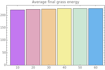
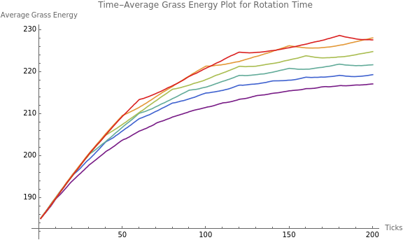
Next, I tested rotation time, which is the number of ticks until the cows move to the next paddock. I used the same process to analyze the data.
testrottime[rottime_]:=Module[{},NLCommand["set rotation-time",rottime,"setup"];data=NLDoReport["go","list(health-sum) (energy-sum)",200];{Map[#[[1]]/50&,data],Map[#[[2]]/10000&,data]}]
In[]:=
repeattest2[rottime_]:=Table[testrottime[rottime],10]
In[]:=
NLCommand["set grass-growth-rate",1.0];NLCommand["set number-of-cows",50];NLCommand["set number-of-regions",2];
In[]:=
time1=repeattest2[10];time2=repeattest2[20];time3=repeattest2[30];time4=repeattest2[40];time5=repeattest2[50];time6=repeattest2[60];
In[]:=
timedata={time1,time2,time3,time4,time5,time6};healthdata2=Map[finalhealth[#]&,timedata];energydata2=Map[finalenergy[#]&,timedata];timeenergy=Map[Mean[#]&,energydata2];timehealth=Map[Mean[#]&,healthdata2];
Out[]=
Health | ||||||||||||||||||||||||||||||||||||||||||||||||||||||||||||||||||||||||||||||||||||
| ||||||||||||||||||||||||||||||||||||||||||||||||||||||||||||||||||||||||||||||||||||
Energy | ||||||||||||||||||||||||||||||||||||||||||||||||||||||||||||||||||||||||||||||||||||
|
In[]:=
BarChart[timeenergy,PlotLabel"Average final grass energy",ChartLabelsRange[10,60,10],ChartStyle"Pastel",FrameTrue]
Out[]=
In[]:=
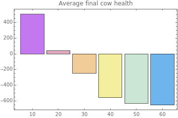
BarChart[timehealth,PlotLabel"Average final cow health",ChartLabelsRange[10,60,10],ChartStyle"Pastel",FrameTrue,AxesLabel"Cow Health"]
Out[]=
allhealth2=Map[fullhealthdata[#]&,timedata];allenergy2=Map[fullenergydata[#]&,timedata];
In[]:=
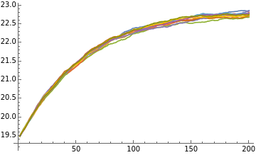
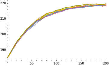
Map[ListLinePlot[#]&,allhealth2]
Out[]=
,
,
,
,
,
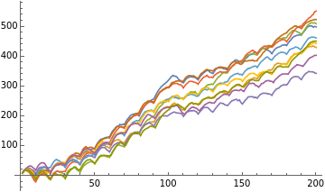
In[]:=
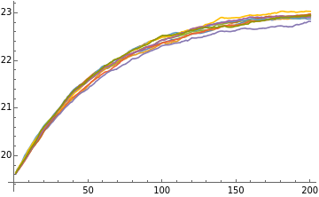
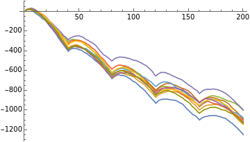
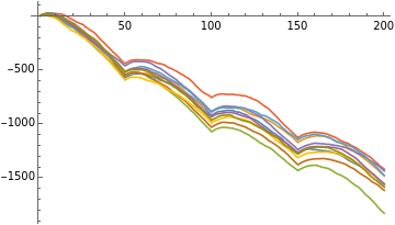
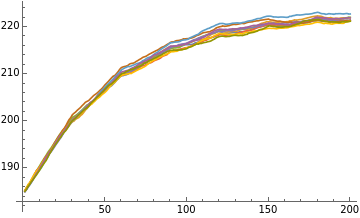
Map[ListLinePlot[#]&,allenergy2]
Out[]=
,
,
,
,
,
healthticks2=Map[Transpose[#]&,allhealth2];energyticks2=Map[Transpose[#]&,allenergy2];
Out[]=
Out[]=
Results
Results
From the data, we can conclude that rotational grazing is more productive than continuous grazing since the final average cow health and grass energy were higher for 2 paddocks than for 1 paddock, but too many paddocks can also be problematic. We also found that a short rotation period is more productive than long rotation periods. The current model is effective to study correlational relationships between the variables, but further development is required for it to simulate more realistic conditions and allow for more factors to be modified and measured. This model does not account for all factors in rotational grazing and it assumes some variable conditions remain constant.
Such variable conditions include:
• Weather: affects grass growth and animal activity
• Grass growth rate
• Grass and soil quality
• Age and health level of cows:reproduction, death, and illness ignored
• Food absorption and energy levels in grass
• Rotation period: typically changing according to forage conditions
• Seasonal changes
• Shape of paddocks
References
References
I apologize that the explanation and code are not very clear and organized, but I thought it would be interesting to share ways of how data from NetLogo can be analyzed in Wolfram. Here are some sources that I used:
◼
[1] D.J. Undersander, B. Albert, D. Cosgrove, D. Johnson, and P. Peterson. Pastures for profit: A guide to rotational grazing. Cooperative Extension Publications, University of Wisconsin-Extension, 2002.
◼
[2] M. Chen and J. Shi. Effect of rotational grazing on plant and animal production. Mathematical Biosciences and Engineering, 15(2):393–406, 2018.
◼
[3] I. Noy-Meir. Rotational grazing in a continuously growing pasture: a simple model. Agricultural Systems, 1(2):87–112, 1976.
◼
[4] U. Wilensky. Netlogo. http://ccl.northwestern.edu/netlogo/, Center for Connected Learning and Computer-Based Modeling, Northwestern University, Evanston, IL, 1999.
◼
[5] S. Tisue and U. Wilensky. Netlogo: A simple environment for modeling complexity. In International conference on complex systems, volume 21, pages 16–21. Boston, MA, 2004.
◼
[6] R. Grider, N. Payette, C. Bain, and E. Landau. Many regions example.nlogo. https://github.com/NetLogo/models/blob/master/CodeExamples/ManyRegionsExample.nlogo, 2016.
For those who are interested, here are the links to NetLogo and the NetLogo-Mathematica Link that I used for this project.
CITE THIS NOTEBOOK
CITE THIS NOTEBOOK
Modeling the maximum potential of rotational grazing with Netlogo
by Jessica Shi
Wolfram Community, STAFF PICKS, 2020
https://community.wolfram.com/groups/-/m/t/1908383
by Jessica Shi
Wolfram Community, STAFF PICKS, 2020
https://community.wolfram.com/groups/-/m/t/1908383