The Wolfram Quantum Framework provides a broad and coherent design for any quantum computation in a finite-dimensional space. Given a quantum query (such as a quantum circuit), there are many different ways that one can communicate with available Quantum Processing Units (QPUs), eg via Wolfram's service connect for AWS. Recently, we have added IBM-quantum as a service connect into the Wolfram quantum framework. In this short computational essay, I will show how to use IBMQ service connect in a Wolfram notebook.
Wolfram quantum framework now comes with the IBM-Q service. You can use ServiceConnect to send queries to IBM quantum hardware and get results
Note you should install Wolfram quantum paclet first (see the initialization section this notebook, first)
Note you should install Wolfram quantum paclet first (see the initialization section this notebook, first)
Initialization cells
Initialization cells
Install Wolfram quantum framework paclet, and load it:
PacletInstall["Wolfram/QuantumFramework"](*PacletInstall["https://wolfr.am/DevWQCF",ForceVersionInstall -> True]this is the developer version, being updated more often that paclet page*)Needs["Wolfram`QuantumFramework`"]
I recognize that the steps mentioned below might seem a bit cumbersome, but make sure you go through them, before anything else.
Note for IBM QPUs, you need Python (make sure to register Python as an external evaluator).
You should also install qiskit package (eg on terminal: pip install qiskit), and qiskit-ibm-provider (eg on terminal: pip install qiskit-ibm-provider).
You can use ResourceFunction["PythonPackageInstall"] to install any python package, too
You should also install qiskit package (eg on terminal: pip install qiskit), and qiskit-ibm-provider (eg on terminal: pip install qiskit-ibm-provider).
You can use ResourceFunction["PythonPackageInstall"] to install any python package, too
ResourceFunction["PythonPackageInstall"]["qiskit"]ResourceFunction["PythonPackageInstall"]["qiskit-ibm-provider"]
These are packages that external evaluator will be using.
Additionally, you should create an IBM-Q account, and get your token
Then run below code using your API token (this is a Python, to save your credentials)
Then run below code using your API token (this is a Python, to save your credentials)
from qiskit_ibm_provider import IBMProvider
IBMProvider.save_account(token='MY_API_TOKEN',overwrite=True)
IBMProvider.save_account(token='MY_API_TOKEN',overwrite=True)
After evaluating above Py code, you can get your token as follow (since it is saved now):
In[]:=
Import["~/.qiskit/qiskit-ibm.json","RawJSON"]["default-ibm-quantum","token"]
Connecting to IBM-quantum
Connecting to IBM-quantum
Using your token, you can connect to IBM-quantum:
In[]:=
ibm=ServiceConnect["IBMQ"]
Out[]=

To make sure you are connected, evaluate the following cell (it will return your account info):
In[]:=
ibm["Account"]
If the outcome was not what you expected, it means you are not connected. So try again using:
ibm=ServiceConnect["IBMQ","New"]
List of requests:
In[]:=
ibm["Requests"]
Out[]=
{Account,Authentication,Backend,BackendQueue,Backends,Devices,ID,Information,JobResults,JobStatus,Name,RawRequests,RunCircuit}
Return the service info:
In[]:=
ibm["Information"]
Out[]=
IBMQ connection for WolframLanguage
List of devices (note some of them are simulator and some are actual QPU):
In[]:=
ibm["Devices"]
Out[]=
ibm-q{ibmq_qasm_simulator,ibmq_quito,ibmq_lima,ibmq_belem,simulator_extended_stabilizer,simulator_mps,simulator_statevector,simulator_stabilizer,ibmq_manila,ibm_oslo,ibm_nairobi,ibm_lagos,ibm_perth,ibmq_jakarta}
List of backends (note some of them are simulator and some are actual QPU):
In[]:=
ibm["Backends"]//Normal
Out[]=
devices{ibmq_manila,ibm_oslo,ibm_nairobi,ibmq_quito,ibmq_lima,ibmq_belem,simulator_mps,simulator_stabilizer,simulator_statevector,ibm_perth,ibmq_jakarta,ibmq_qasm_simulator,simulator_extended_stabilizer,ibm_lagos}
You can also get more info on each one. For example:
ibm["Backend","ID"->XXX,"Property"->"Properties"]
ibm["Backend","ID"->XXX,"Property"->"Configuration"]
ibm["Backend","ID"->XXX,"Property"->"Status"]
ibm["Backend","ID"->XXX,"Property"->"Defaults"]
Get configuration of one backend:
In[]:=
config=ibm["Backend","ID"->"ibmq_belem","Property"->"Configuration"];config//Keys//Normal
Out[]=
{acquisition_latency,allow_q_object,backend_name,backend_version,basis_gates,channels,clops,conditional,conditional_latency,coupling_map,credits_required,default_rep_delay,description,discriminators,dt,dtm,dynamic_reprate_enabled,gates,hamiltonian,local,max_experiments,max_shots,meas_kernels,meas_levels,meas_lo_range,meas_map,measure_esp_enabled,memory,multi_meas_enabled,n_qubits,n_registers,n_uchannels,online_date,open_pulse,parallel_compilation,parametric_pulses,processor_type,quantum_volume,qubit_channel_mapping,qubit_lo_range,rep_delay_range,rep_times,sample_name,simulator,supported_features,supported_instructions,timing_constraints,u_channel_lo,uchannels_enabled,url}
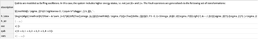
Return Hamiltonian description:
In[]:=
config["hamiltonian"]
Out[]=
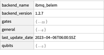
Or one can get properties:
In[]:=
prop=ibm["Backend","ID"->"ibmq_belem","Property"->"Properties"]
Out[]=
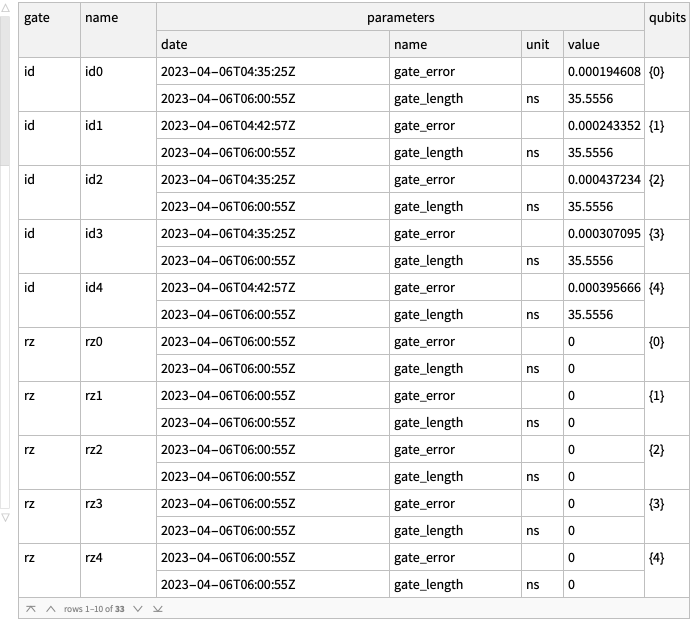
Some info on errors:
In[]:=
prop["gates"]
Out[]=
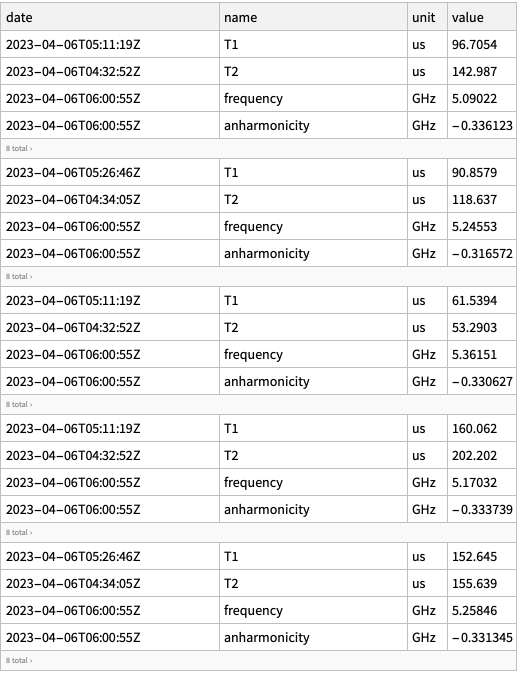
In[]:=
prop["qubits"]
Out[]=
Designing a quantum circuit
Designing a quantum circuit
For example, let’s consider a 4-qubit circuit for creating a random pure state. This is a circuit one can use to generate random discrete numbers with a desired probability. For more info, see this project from Wolfram Winter School 2023.
For simplicity, we will create a random pure state with real amplitudes, rather complex (a generic random state can be created by QuantumState[{“RandomPure”,n}])
In[]:=
qc=With[{n=4},QuantumCircuitOperator[r=QuantumState[{"RandomPure",n}]]/*QuantumMeasurementOperator[Range[n]]];
Return the state vector of the 4-qubit pure state generated randomly:
In[]:=
r["StateVector"]//Normal
Out[]=
{-0.176454-0.269641,-0.312244-0.13172,-0.1936+0.174401,-0.0739316+0.0847887,0.252453-0.0962371,-0.0638498+0.0025841,0.315675+0.415406,0.0671476+0.0337656,0.216087-0.0502779,0.0165728+0.00598322,-0.054711+0.0507679,-0.380085-0.168748,0.0972689-0.0811526,0.17107+0.0841524,-0.101599+0.107732,-0.118983+0.171164}
Return circuit diagram:
In[]:=
qc["Diagram","ShowGateLabels"->False]
Out[]=
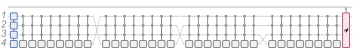
Return list of all gates in above circuit (note the multiplexer are composition of rotation operators, see below result)
In[]:=
QuantumLabelName[qc]
Out[]=
Note if you wrap above output (list of labels) as a circuit, you will get the original circuit:
In[]:=
QuantumCircuitOperator[%]==qc
Out[]=
True
Transform the circuit into qiskit object, then decompose it
If you do not decompose, qiskit transpiler may have some issues with multiplexers (note in the example, I am using, we usually have multiplexer)
If any issue, try simpler circuits that qiski transpiler can handle
If you do not decompose, qiskit transpiler may have some issues with multiplexers (note in the example, I am using, we usually have multiplexer)
If any issue, try simpler circuits that qiski transpiler can handle
In[]:=
qiskit=qc["Qiskit"]["Decompose"];
Turn the qiskit object into bytes by specifying the corresponding provider and backend on IBM system (this step may take long)
Note I have chosen “ibmq_belem” as the backend, because when I was writing these codes, it was the QPUs with the list number of queue
Note I have chosen “ibmq_belem” as the backend, because when I was writing these codes, it was the QPUs with the list number of queue
In[]:=
qpy=BaseEncode@qiskit["QPY","Provider"->"IBMProvider","Backend"->"ibmq_belem"];
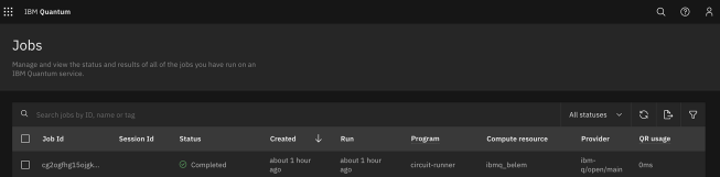
Send the circuit to an IBM QPU (note that the JobID will be different for each user):
In[]:=
ibm["RunCircuit",{"QPY"->qpy,"Backend"->"ibmq_belem"}]
Out[]=
Users should pay attention to specs of each QPUs eg gates they accept or number of qubits etc (see the last section in this notebook for more details)
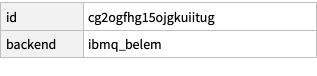
Check the job’s status (note that the JobID will be different for each user; and the job will take some time to be completed):
In[]:=
ibm["JobStatus",{"JobID"->"cg2ogfhg15ojgkuiitug"}]
Out[]=
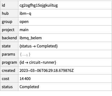
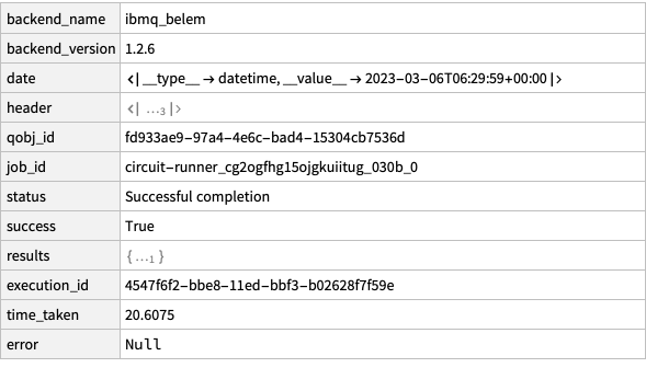
Get the results (it takes some time to get the result):
In[]:=
ds=ibm["JobResults",{"JobID"->"cg2ogfhg15ojgkuiitug"}]
Out[]=
Given counts in the results, find the corresponding probabilities:
In[]:=
Normal[ds["results",All,"data","counts"]][[1]]
Out[]=
0x0463,0x1257,0x2357,0x3197,0x4433,0x5182,0x6316,0x7144,0x8332,0x9178,0xa236,0xb120,0xc256,0xd175,0xe241,0xf113
In[]:=
qpuResults=N@Normalize[Values@%,Total]
Out[]=
{0.11575,0.06425,0.08925,0.04925,0.10825,0.0455,0.079,0.036,0.083,0.0445,0.059,0.03,0.064,0.04375,0.06025,0.02825}
Get the results from Wolfram quantum framework (exact results):
In[]:=
results=qc[]["Probabilities"]
Out[]=
|0000〉0.103842,|0001〉0.114847,|0010〉0.0678967,|0011〉0.012655,|0100〉0.072994,|0101〉0.00408348,|0110〉0.272213,|0111〉0.00564891,|1000〉0.0492216,|1001〉0.000310457,|1010〉0.00557067,|1011〉0.172941,|1100〉0.016047,|1101〉0.0363467,|1110〉0.0219285,|1111〉0.0434543
BarChart[Transpose[{Values[results],qpuResults}],ChartLegends->{"Wolfram quantum framwork","IBM QPU"}]
Out[]=
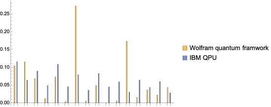
Note that the results from Wolfram quantum framework are the ones predicted by quantum theory. As one can see, there has been some errors in the hardware (maybe due to environmental noises or other effects).
If any question or comment, please contact us at: quantum AT wolfram.com
CITE THIS NOTEBOOK
CITE THIS NOTEBOOK
Wolfram Quantum Framework: IBM-quantum service connect
by Mohammad Bahrami
Wolfram Community, STAFF PICKS, March 7, 2023
https://community.wolfram.com/groups/-/m/t/2846060
by Mohammad Bahrami
Wolfram Community, STAFF PICKS, March 7, 2023
https://community.wolfram.com/groups/-/m/t/2846060