Huge congratulations to John Clarke, Michel H. Devoret, and John M. Martinis on the 2025 Nobel Prize in Physics “for the discovery of macroscopic quantum mechanical tunnelling and energy quantisation in an electric circuit.” Their superconducting Josephson-circuit experiments made quantum effects unmistakably visible at circuit scale, discrete, anharmonic energy levels and coherent tunnelling between macroscopically distinct states, laying key groundwork for modern superconducting qubits. In this short computational essay, we’ll walk through compact simulations that reproduce those signatures: a spectroscopy-style level map for the Cooper-pair box/transmon, and time-domain tunnelling dynamics with realistic decoherence to mirror the original observations.
Energy quantization in a Josephson circuit (Cooper-pair box / transmon toy)
Energy quantization in a Josephson circuit (Cooper-pair box / transmon toy)
A small superconducting island, linked by a Josephson junction and capacitively coupled to a gate, is described by conjugate variables: the superconducting phase across the junction and the integer number of Cooper pairs on the island. The key energy scales are the charging energy set by the island capacitance, the Josephson energy set by the junction’s critical current, and the offset charge controlled by the gate. In the charge basis the Hamiltonian becomes a real, symmetric, tridiagonal matrix with a diagonal charging term and nearest-neighbor couplings from the cosine Josephson term; diagonalization yields discrete, anharmonic energy levels. As the ratio of Josephson to charging energy increases, the device evolves from a charge-qubit regime with strong offset-charge dispersion and prominent avoided crossings near half-integer offset to a transmon regime with suppressed dispersion and a weakly anharmonic ladder whose anharmonicity is set by the charging scale. Microwave spectroscopy versus gate offset (or flux in related devices) reveals these discrete transitions and their anharmonicity, while linewidths report the underlying coherence times.
Consider the Hamiltonian as =4--cos with the Cooper-pair number with integer eigenvalues, and ϕ the superconducting phase across the junction. They are canonically conjugate: and =-. Additionally, is the charging energy, is the Josephson energy, and is the gate offset charge. The Hamiltonian can be considered as a quantum rotor (phase) in a cosine potential, minimally coupled to a static “vector potential” that shifts the momentum .
H
2
E
C
n
n
g
E
J
ϕ
n
,=
ϕ
n
n
∂
∂ϕ
E
C
E
J
n
g
n
g
n
The charge basis is denoted as with |n〉=n|n〉. The phase operator acts as a ladder in this basis: |n〉=|n∓1〉. Thus, this implies . Put all of these together, the Hamiltonian can be described in a truncated space, by setting
{|n〉}
nϵ
n
±
ϕ
cos=(|n〉〈n+1|+|n+1〉〈n|)
ϕ
1
2
∑
n
-<=n<=
n
max
n
max
In[]:=
ClearAll[hamiltonian];hamiltonian[ratio_,ng_,nmax_:20]:=DiagonalMatrixTable4,{n,-nmax,nmax}-SparseArray[{Band[{1,2}]1,Band[{2,1}]1},{2nmax+1,2nmax+1}]
2
(n-ng)
ratio(*EJ/EC*)
2
Given above Hamiltonian (truncated version, find eigenvalues as a function of ):
n
g
In[]:=


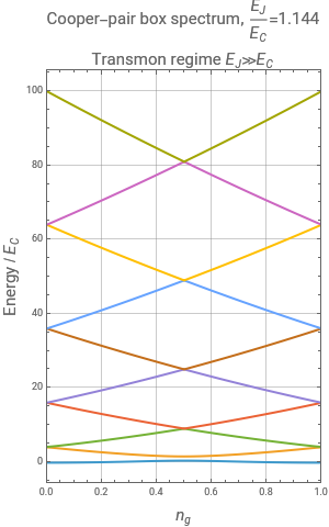
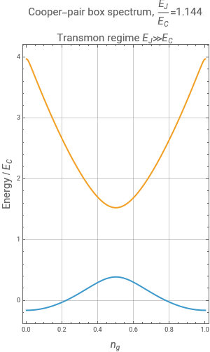
The level curvature and avoided crossings reflect Josephson coupling, direct evidence of quantized levels in an electric circuit (a key piece of the laureates’ work).
Macroscopic quantum tunnelling (two-level double-well model)
Macroscopic quantum tunnelling (two-level double-well model)
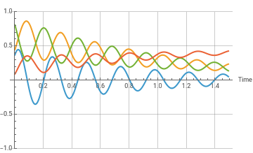
Superconducting circuits can realize an effective double-well potential in phase or flux, hosting states localized in left and right wells that are macroscopically distinct. Restricting to the two lowest localized states gives a minimal model with a tunnel coupling, which mixes the wells, and a tunable bias, which tilts their relative energies. If the system is prepared in one well, the population coherently oscillates between wells with a frequency set by the combined effect of coupling and bias and with an amplitude that is maximal at symmetry and decreases as the bias grows. Pure dephasing damps the oscillation contrast, energy relaxation drives the system toward the lower-energy well’s stationary population, and finite temperature can repopulate the higher level; the observed coherence time reflects both relaxation and dephasing. Time-domain oscillations, spectroscopy of the bias-dependent splitting near symmetry, and escape-rate or switching-current measurements that crossover from thermal activation at high temperature to temperature-independent quantum tunnelling at low temperature together provide the experimental fingerprints of this macroscopic quantum behavior.
Let’s define a two-level system by the Hamiltonian :
H=+
ϵ
2
σ
z
Δ
2
σ
x
In[]:=
$Assumptions={ϵ,Δ}>0;h=PauliMatrix[3]+PauliMatrix[2];h//MatrixForm
ϵ
2
Δ
2
Out[]//MatrixForm=
ϵ 2 | - Δ 2 |
Δ 2 | - ϵ 2 |
Here ϵ represents the bias (tilt) between wells, and Δ is the tunnel splitting.
Find the eigenvalues of the Hamiltonian:
In[]:=
{,}=Eigenvalues[h]
ℰ
1
ℰ
2
Out[]=
-+,+
1
2
2
Δ
2
ϵ
1
2
2
Δ
2
ϵ
Given above result, is usually called the eigenfrequency.
Ω=+
2
Δ
2
ϵ
In[]:=
{,}=Normalize/@Eigenvectors[h]
e
1
e
2
Out[]=
,,-,
-ϵ++
2
Δ
2
ϵ
Δ
1+
2
Abs
-ϵ++
2
Δ
2
ϵ
Δ
1
1+
2
Abs
-ϵ++
2
Δ
2
ϵ
Δ
ϵ++
2
Δ
2
ϵ
Δ
1+
2
Abs
ϵ++
2
Δ
2
ϵ
Δ
1
1+
2
Abs
ϵ++
2
Δ
2
ϵ
Δ
Set the initial state at the bottom of one of the wells (i.e., the eigenstate of ):
σ
z
In[]:=
ψ
0
Using the Schrodinger equation, find the final state at a given time:
In[]:=
ψ[t_]=Exp[-It].//FullSimplify
2
∑
i=1
ℰ
i
e
i
ψ
0
e
i
Out[]=
Cost+-+,+
1
2
2
Δ
2
ϵ
ϵSint+
1
2
2
Δ
2
ϵ
2
Δ
2
ϵ
ΔSint+
1
2
2
Δ
2
ϵ
2
Δ
2
ϵ
Calculate the probability of tunneling:
In[]:=
{0,1}.ψ[t]{0,1}.ψ[t]//FullSimplify
Out[]=
2
Δ
2
Sint+
1
2
2
Δ
2
ϵ
2
Δ
2
ϵ
The above behavior assumes coherent tunneling, i.e., no noise. In practice, environmental interactions introduce dephasing, relaxation, and other channels, so the dynamics deviate from the Schrödinger equation and the qubit becomes an open system. A common model for such open-system dynamics is the Lindblad master equation:
∂
t
∑
k
L
k
[][ρ]=ρ-,ρ
L
k
L
k
†
L
k
1
2
†
L
k
L
k
with the corresponding Lindblad/jump operators.
L
k
Define the Lindblad terms:
In[]:=
ClearAll[][L_,ρ_]:=L.ρ.ConjugateTranspose[L]-(ConjugateTranspose[L].L.ρ+ρ.ConjugateTranspose[L].L)
1
2
For the case of energy relaxation (downward transitions), we have:
∂
t
σ
-
ρσ
+
1
2
σ
+
σ
-
γ=1/
T
1
For the case of pure dephasing (phase randomization without energy exchange), one gets:
∂
t
Γ
ϕ
2
σ
z
ρσ
z
Γ
ϕ
T
ϕ
Putting them together, the total transverse coherence (T₂) combines both mechanisms =+
1
T
2
1
2
T
1
1
T
ϕ
Define a vector such that where 3-vector is usually called the Bloch vector:
ρ=(+.)
1
2
r
σ
r
r={1,rx[t],ry[t],rz[t]};
Note the transformation from Bloch vector in the Cartesian coordinate to spherical and vice versa:
In[]:=
CoordinateTransformData"Cartesian""Spherical","Mapping",x.,y.,z.
Out[]=
++,ArcTanz.,+,ArcTan[x.,y.]
2
x.
2
y.
2
z.
2
x.
2
y.
In[]:=
CoordinateTransformData"Spherical"->"Cartesian","Mapping",r.,θ,ϕ//FullSimplify
Out[]=
r.Cos[ϕ]Sin[θ],r.Sin[θ]Sin[ϕ],r.Cos[θ]
Find the density matrix:
ρ=r.Table[PauliMatrix[j],{j,0,3}]//FullSimplify;ρ//MatrixForm
1
2
Out[]//MatrixForm=
1 2 | 1 2 |
1 2 | 1 2 |
Define the jump operator for relaxation:
In[]:=
σs={{0,0},{0,1}};
Put relaxation and pure dephasing together into dynamical equation:
In[]:=
dρt=-(h.ρ-ρ.h)+γ[σs,ρ]+[PauliMatrix[3],ρ]//FullSimplify
Γϕ
2
Out[]=
-Δrx[t],(-((γ+2Γϕ+2ϵ)(rx[t]-ry[t]))+2Δrz[t]),(-((γ+2Γϕ-2ϵ)(rx[t]+ry[t]))+2Δrz[t]),Δrx[t]
1
2
1
4
1
4
1
2
Given the evolution of the density matrix, find the evolution of the Bloch vector:
In[]:=
drt=Table[Tr[dρt.PauliMatrix[j]]//FullSimplify,{j,3}]
Out[]=
-(γ+2Γϕ)rx[t]-ϵry[t]+Δrz[t],ϵrx[t]-(γ+2Γϕ)ry[t],-Δrx[t]
1
2
1
2
Set the dynamical equations and the initial conditions:
In[]:=
eqns=Thread[D[{rx[t],ry[t],rz[t]},t]==drt]ic={rx[0]==rx0,ry[0]==ry0,rz[0]==rz0}
Out[]=
[t]-(γ+2Γϕ)rx[t]-ϵry[t]+Δrz[t],[t]ϵrx[t]-(γ+2Γϕ)ry[t],[t]-Δrx[t]
′
rx
1
2
′
ry
1
2
′
rz
Out[]=
{rx[0]rx0,ry[0]ry0,rz[0]rz0}
Put all of them into a parametric DEs:
In[]:=
pnd=ParametricNDSolveValue[Join[eqns,ic],{rx,ry,rz},{t,0,T},{rx0,ry0,rz0,Δ,γ,Γϕ,ϵ,T}]
Out[]=
ParametricFunction
Visualize the parametric DEs, for different values of the corresponding parameters:
Out[]=

CITE THIS NOTEBOOK
CITE THIS NOTEBOOK
Nobel Prize in Physics 2025: Macroscopic Quantum Effects and the Dawn of Quantum Computer
by Mohammad Bahrami
Wolfram Community, STAFF PICKS, October 8, 2025
https://community.wolfram.com/groups/-/m/t/3558195
by Mohammad Bahrami
Wolfram Community, STAFF PICKS, October 8, 2025
https://community.wolfram.com/groups/-/m/t/3558195