The purpose of this project was to be able to develop a system that can track satellites over time and model their collisions if they occur. I began by using a differential equation solver that could track the motion of satellites under the influence of gravity. I used this approach to model a simple collision in space. I then created an NBodySimulation that has the ability to track multiple satellites, their collisions, and their paths.
Introduction
Introduction
As with many other things, as soon as humans discovered space, we have been creating a mess. In 1957 the Soviet Union launched the first satellite, Sputnik. Since then, year after year, we have been progressively launching more satellites. Orbiting our planet are thousands of satellites, dead satellites, and space debris. NASA estimates that there are roughly 500,000 objects between 1 and 10 centimeters in diameter orbiting Earth. The Department of Defense's global Space Surveillance Network (SSN) sensors track over 27,000 pieces of orbital debris. Every year there are multiple near collisions between satellites or pieces of debris. In 2021 Russia blew up a dead satellite creating a massive debris field that threatened the International Space Station. If nothing is done to fix this issue, Earth's orbit could become so polluted it would be unsafe for human exploration resulting in a phenomenon called Kessler Syndrome.
Kessler Syndrome happens when the amount of debris around the Earth reaches a point where it creates more and more space debris resulting in a cascading effect that leads to millions of pieces of debris around the Earth. This would hinder future space ambitions, resulting in a nightmarish scenario where humans would be trapped on Earth.
Kessler Syndrome happens when the amount of debris around the Earth reaches a point where it creates more and more space debris resulting in a cascading effect that leads to millions of pieces of debris around the Earth. This would hinder future space ambitions, resulting in a nightmarish scenario where humans would be trapped on Earth.
Differential Equations Method
Differential Equations Method
Defining Global Constants
Defining Global Constants
To begin, I needed to define global constants that would be used in future functions. According to NASA, the radius of the Earth is 6371 km which is 6,371,000 Meters. G is the gravitational constant found by Lord Henry Cavendish. M is the mass in kilograms of the Earth.
In[]:=
earthRadius=6371000;G=6.673*10^-11;M=5.98*10^24;
Differential Equations Function
Differential Equations Function
The primary force that acts on a satellite is the force of gravity from the Earth. Differential equations can be used to model the movement of satellites under the influence of gravity. Differential equations are mathematical equations that involve one or more unknown functions and their derivatives(rates of change). They describe relationships between the derivatives and the function itself. These equations are widely used in many fields, including physics, engineering, economics, biology, and computer science, to model various phenomena and predict their behavior over time.We can model the movement of satellites by using their acceleration which is determined by the equation below. From this, we want to determine the position functions of a satellite.
g=
-GM
2
r
r
In this equationg = gravitational accelerationG = gravitational constantM = Mass of the Earthr = distance between the two point like masses = a unit vector directed from the Earth to the satelliteWe can adapt this to the acceleration in the {x,y,z} direction. r, the distance between two points, is the magnitude at each point in time. is the unit vector, so it is the component over the magnitude of the vector.Thus, the acceleration of the x component it results ina = ++×++This can be used for the y and z components as well.Acceleration is the 2nd derivative of position, and thus using acceleration, an initial position, and an initial velocity, we can determine position functions.
r
r
-GM
2
x[t]
2
y[t]
2
z[t]
x[t]
2
x[t]
2
y[t]
2
z[t]
-GM(x[t])
3/2
++
2
x[t]
2
y[t]
2
z[t]
Below I begin by using NDSolve to solve the differential equations described above, given an initial position and velocity. This returns a function with the domain from t = 0 to t = 100000
NDSolve returns {x[t],y[t],z[t]} functions given initial position and velocity:
In[]:=
sol[x0_,y0_,z0_,v0x_,v0y_,v0z_]:=Flatten[NDSolve[{x''[t]==-G*M((x[t])/(x[t]^2+y[t]^2+z[t]^2)^(3/2)),y''[t]==-(G*M(y[t])/(x[t]^2+y[t]^2+z[t]^2)^(3/2)),z''[t]==-G*M((z[t])/(x[t]^2+y[t]^2+z[t]^2)^(3/2)),x[0]==x0,y[0]==y0,z[0]==z0,x'[0]==v0x,y'[0]==v0y,z'[0]==v0z},{x[t],y[t],z[t]},{t,0,100000}]];
Plot of the Orbit using a Differential Equation
Plot of the Orbit using a Differential Equation
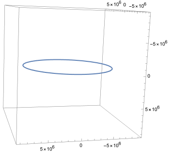
This is an example of the differential equation solver being used with a known orbit. This is the orbit of an object around the Earth {0,0,0}, initialized with an altitude of 1000 meters and with an initial velocity that produces a circular orbit. Given my differential equation solver, I wanted to test it against known orbits. I aimed to plot a simple circular horizontal orbit.You can calculate a perfectly circular orbit by setting the centripetal force experienced by an object equal to the gravitational force. In this equationm = mass of the satellitev = orbital velocityr = radius from Earth to satelliteG = gravitational constantM = mass of the EarthSolving for v results inSubbing a point at a radius of 7371000 meters results in a velocity of 7357. I set the initial position to {7371000,0,0} and determined the initial velocity would only be in the y direction.
2
mv
r
GMm
2
r
v
GM
r
The differential equation solver uses these points and then ParametricPlot3D plots the resulting function:
In[]:=
ParametricPlot3D[Evaluate[{x[t],y[t],z[t]}/.sol[7371000,0,0,0,-7357,0]],{t,1,10000},PlotRange->{{-earthRadius*1.5,earthRadius*1.5},{-earthRadius*1.5,earthRadius*1.5},{-earthRadius*1.5,earthRadius*1.5}}]
Out[]=
Animating multiple satellites using the Differential Equation Method
Animating multiple satellites using the Differential Equation Method
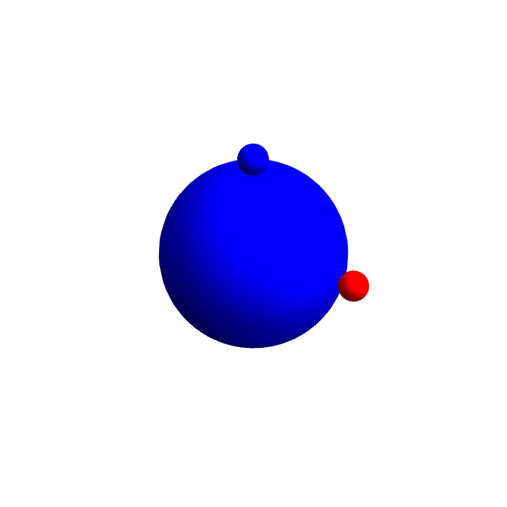
Similarly to above, I aimed to plot both a horizontal and vertical satellite.
Evaluates the position function for a horizontal and vertical satellite:
In[]:=
sat1=Evaluate[{x[t],y[t],z[t]}/.sol[7371000,0,0,0,-7357,0]];sat2=Evaluate[{x[t],y[t],z[t]}/.sol[0,0,7371000,0,-7357,0]];
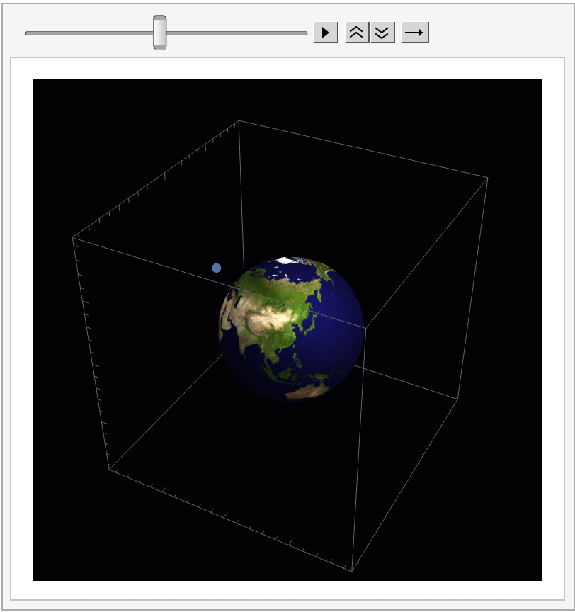
I wanted to animate these two satellites to see their motion over time. I used graphics and table to create a list of the satellites at different times. I then used ListAnimate to animate over those points.
Creates a table of 2 satellites,their positions and the Earth. Then uses ListAnimate to create an animation:
In[]:=
frames=Table[Graphics3D[{Blue,Sphere[{0,0,0},earthRadius],(*satellite*)Red,Sphere[sat1,1000000(*radiusofSatellite*)],(*satellite*)Blue,Sphere[sat2,1000000(*radiusofSatellite*)]},Boxed->False,Lighting->"Neutral",PlotRange->{{-earthRadius*1.5,earthRadius*1.5},{-earthRadius*1.5,earthRadius*1.5},{-earthRadius*1.5,earthRadius*1.5}},SphericalRegion->True,ViewAngle->All],{t,0,10000,100}];ListAnimate[frames]
Out[]=
Simple collision with the Differential Equation Approach
Simple collision with the Differential Equation Approach
Check Tolerance Function
Check Tolerance Function
This function will check whether 2 satellites are colliding. For simplicity reasons a collision is determined is 2 satellites are within 200,000 meters of each other. (This will be updated to a much smaller number later do not worry)
In[]:=
equaltolerance[n_,x_]:=If[Norm[n-x]<200000,True,False]
Conserving Momentum Function
Conserving Momentum Function
Conservation of momentum states that the amount of momentum following a collision is the same as before the collision.
This function uses the basic principle of conservation of momentum. It takes in 2 colliding satellites and returns 4 new satellites The masses of the 4 satellites are evenly spread, and the velocities are randomly generated while adhering to the rules of conservation of momentum.
This function uses the basic principle of conservation of momentum. It takes in 2 colliding satellites and returns 4 new satellites The masses of the 4 satellites are evenly spread, and the velocities are randomly generated while adhering to the rules of conservation of momentum.
Takes in 2 masses and the velocity components of 2 satellites and returns masses and velocities for 4 new satellites:
In[]:=
momentumfind[m1_,m2_,v1x_,v1y_,v1z_,v2x_,v2y_,v2z_]:=FindInstance[{m1*v1x,m1*v1y,m1*v1z}+{m2*v2x,m2*v2y,m2*v2z}{m3*v3x,m3*v3y,m3*v3z}+{m4*v4x,m4*v4y,m4*v4z}+{m5*v5x,m5*v5y,m5*v5z}+{m6*v6x,m6*v6y,m6*v6z}&&m3==(m1+m2)/4&&m4==(m1+m2)/4&&m5==(m1+m2)/4&&m6==(m1+m2)/4&&m3>0&&Sqrt[v3x^2+v3y^2+v3z^2]>3000&&Sqrt[v4x^2+v4y^2+v4z^2]>3000&&Sqrt[v5x^2+v5y^2+v5z^2]>3000,{m3,v3x,v3y,v3z,m4,v4x,v4y,v4z,m5,v5x,v5y,v5z,m6,v6x,v6y,v6z},Reals,2]
Randomizes the previous function:
In[]:=
momentumfindrand[m1_,m2_,v1x_,v1y_,v1z_,v2x_,v2y_,v2z_]:=momentumfind[m1,m2,v1x,v1y,v1z,v2x,v2y,v2z][[1]]
Checking if Two Satellites Hit each other
Checking if Two Satellites Hit each other
Next I had to make a function that would check if 2 satellites were going colliding and return 4 new satellites.
Takes in the masses of 2 satellites and their position and the time and returns 4 new satellites if it was a collision:
In[]:=
Overlapcheck[m1_,m2_,p1_,p2_,tp_]:=If[equaltolerance[(p1/.t->tp),(p2/.t->tp)],v1x=D[p1[[1]],t]/.t->tp;v1y=D[p1[[2]],t]/.t->tp;v1z=D[p1[[3]],t]/.t->tp;v2x=D[p2[[1]],t]/.t->tp;v2y=D[p2[[2]],t]/.t->tp;v2z=D[p2[[3]],t]/.t->tp;momentumfindrand[m1,m2,v1x,v1y,v1z,v2x,v2y,v2z]]
Combining for Animation
Combining for Animation
The next step was combining all these functions and creating a very simple collision. I began by determining the time the 2 satellites would collide and the new velocities of the satellites following the collision.
Finds the time the horizontal and vertical satellites collide and then maps their velocities and masses to a list:
In[]:=
timehit=Select[Table[If[equaltolerance[(sat1/.t->i),(sat2/.t->i)],i],{i,0,10000}],IntegerQ][[1]];v={m3,v3x,v3y,v3z,m4,v4x,v4y,v4z,m5,v5x,v5y,v5z,m6,v6x,v6y,v6z}/.Overlapcheck[100,100,sat1,sat2,timehit];ls={m3,v3x,v3y,v3z,m4,v4x,v4y,v4z,m5,v5x,v5y,v5z,m6,v6x,v6y,v6z};MapThread[Set,{ls,v}];
Defining the new satellites given their parameters:
In[]:=
sat3=Evaluate[{x[t],y[t],z[t]}/.sol[(sat1/.t->timehit)[[1]],(sat1/.t->timehit)[[2]],(sat1/.t->timehit)[[3]],v3x,v3y,v3z]];sat4=Evaluate[{x[t],y[t],z[t]}/.sol[(sat1/.t->timehit)[[1]],(sat1/.t->timehit)[[2]],(sat1/.t->timehit)[[3]],v4x,v4y,v4z]];sat5=Evaluate[{x[t],y[t],z[t]}/.sol[(sat1/.t->timehit)[[1]],(sat1/.t->timehit)[[2]],(sat1/.t->timehit)[[3]],v5x,v5y,v5z]];sat6=Evaluate[{x[t],y[t],z[t]}/.sol[(sat1/.t->timehit)[[1]],(sat1/.t->timehit)[[2]],(sat1/.t->timehit)[[3]],v6x,v6y,v6z]];
Currently, the position functions of the new satellites begin from time 0. However, the collision does not occur at time 0; thus, they have to shift to where the collision occurs
Shifts the satellites by their collision time:
In[]:=
sat3=sat3/.t->t-timehit;sat4=sat4/.t->t-timehit;sat5=sat5/.t->t-timehit;sat6=sat6/.t->t-timehit;
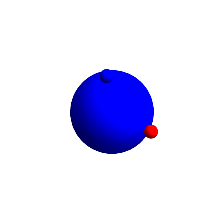
Finally, I wanted to animate the collision and see what was happening through time. I used a similar approach to the above when I plotted the 2 satellites. However, when the time of the collision hits, the expression changes to include the 4 new satellites.
Creates a list of the position of satellites before and after the collision and then animates them:
In[]:=
frames=Table[Which[t<timehit,Graphics3D[{Blue,Sphere[{0,0,0},earthRadius],(*satellite*)Red,Sphere[sat1,1000000(*radiusofSatellite*)],(*satellite*)Blue,Sphere[sat2,1000000(*radiusofSatellite*)]},Boxed->False,Lighting->"Neutral",PlotRange->{{-earthRadius*1.5,earthRadius*1.5},{-earthRadius*1.5,earthRadius*1.5},{-earthRadius*1.5,earthRadius*1.5}},SphericalRegion->True,ViewAngle->All],t>timehit,Graphics3D[{Blue,Sphere[{0,0,0},earthRadius],(*satellite*)Red,Opacity[.5],Sphere[sat3,500000(*radiusofSatellite*)],(*satellite*)Yellow,Opacity[.5],Sphere[sat4,700000(*radiusofSatellite*)],(*satellite*)Pink,Opacity[.5],Sphere[sat5,500000(*radiusofSatellite*)],(*satellite*)Brown,Opacity[.7],Sphere[sat6,300000(*radiusofSatellite*)]},Boxed->False,Lighting->"Neutral",PlotRange->{{-earthRadius*1.5,earthRadius*1.5},{-earthRadius*1.5,earthRadius*1.5},{-earthRadius*1.5,earthRadius*1.5}},SphericalRegion->True,ViewAngle->All]],{t,0,2500,70}];//QuietListAnimate[frames]
Out[]=
In[]:=
ClearAll[m3,v3x,v3y,v3z,m4,v4x,v4y,v4z,m5,v5x,v5y,v5z,m6,v6x,v6y,v6z,sat1,sat2,sat3,sat4,sat5,sat6]
Preparing for a NBody simulation
Preparing for a NBody simulation
The previous approach was great for understanding the movement of satellites and the differential equations behind them. However, it would not scale up great when dealing with multiple satellites. Thus I began a new approach using Wolfram's built-in NBodySimulation function. N-body simulation refers to a computational technique used to model the motion and interactions of a system consisting of multiple particles or bodies. The NBodySimulation function in Wolfram Language allows you to simulate the motion and interactions of multiple bodies under gravitational forces. The NBodySimulation will take in parameters similar to the differential equation solver and will use the same acceleration approach.
Check Tolerance Function
Check Tolerance Function
This function will check whether 2 satellites are colliding. They are declared colliding if the distance between them is less than 4500 meters.
In[]:=
equaltolerance[n_,x_]:=If[Norm[n-x]<4500,True,False]
In[]:=
Collision function
Collision function
This is the collision function that will be used within the NBodySimulation loop later. This will evaluate if it has been determined 2 satellites are colliding. It returns a list of rules that can be inputted back into the NBodySimulation. It generates a RandomString name for new satellites and adds them to the list of bodies that NBodySimulation tracks.
The collision function takes in mass, position, and velocity parameters and returns a list of rules to be appended to bodies NBodySimulation tracks:
In[]:=
collision[m1_Integer,pos1_List,vel1_List,m2_Integer,pos2_List,vel2_List]:=Module[{a,m3,vel3,vel4,m4,m5,vel5,m6,vel6},a=momentumfindrand[m1,m2,vel1[[1]],vel1[[2]],vel1[[3]],vel2[[1]],vel2[[2]],vel2[[3]]];m3=a[[All,2]][[1]];vel3=a[[All,2]][[2;;4]];m4=a[[All,2]][[5]];vel4=a[[All,2]][[6;;8]];m5=a[[All,2]][[9]];vel5=a[[All,2]][[10;;12]];m6=a[[All,2]][[13]];vel6=a[[All,2]][[14;;16]];{ResourceFunction["RandomString"][6]->"Mass"->m3,"Position"->pos1+{0,3556,0},"Velocity"->vel3,ResourceFunction["RandomString"][6]->"Mass"->m4,"Position"->pos1+{3556,0,0},"Velocity"->vel4,ResourceFunction["RandomString"][6]->"Mass"->m5,"Position"->pos1+{-3556,0,0},"Velocity"->vel5,ResourceFunction["RandomString"][6]->"Mass"->m6,"Position"->pos1+{0,-3556,0},"Velocity"->vel6}]
Checks if something is colliding and if so evaluates the collision function:
In[]:=
collisioneval[x_Rule,y_Rule]:=If[equaltolerance[x[[2]]["Position"],y[[2]]["Position"]],collision[x[[2]]["Mass"],x[[2]]["Position"],x[[2]]["Velocity"],y[[2]]["Mass"],y[[2]]["Position"],y[[2]]["Velocity"]]]
These following lines test how the collision function works and what it will return.
While loop using NBody approach
While loop using NBody approach
Clearing all old definitions for satellites:
In[]:=
fulllist={};
In[]:=
ClearAll[sat1];ClearAll[sat2];ClearAll[sat3];ClearAll[sat4];ClearAll[sat5];ClearAll[sat6];
For the NBodySimulation I begin by defining an initial set of satellites. I chose to define X number of satellites. However this simulation can tracks hundreds of satellites.
Initializes a set of satellites used in the NBodySimulation:
In[]:=
set={earth"Mass"5.97219*10^24,"Position"{0,0,0},"Velocity"{0,0,0},sat1"Mass"1,"Position"{7371000,0,0},"Velocity"{0,-7357,0},sat2"Mass"1,"Position"{0,0,7371000},"Velocity"{0,-7357,0},sat3"Mass"1,"Position"{7371100,0,0},"Velocity"{-7357,0,0},sat4"Mass"1,"Position"{7371200,0,0},"Velocity"{0,7357,0},sat5"Mass"1,"Position"{0,0,7371100},"Velocity"{0,7357,0},sat6->"Mass"1,"Position"{7371250,0,0},"Velocity"{0,4729.63123207,5636.55501247},sat7->"Mass"1,"Position"{-4256000,-4256000,-4256000},"Velocity"{-1000,-1000,7500},sat8->"Mass"1,"Position"{7371025,0,0},"Velocity"{0,-4725.13171881,5631.19270137},sat9->"Mass"1,"Position"{-7371025,0,0},"Velocity"{0,-4725.13171881,5631.19270137}};
This is the loop where the NBodySimulation runs. The NBodySimulation is defined using the Newtonian law, which means the simulation will use Newtonian gravity. The set of bodies inputted into the NBodySimulation is constantly updated in the loop. If a satellite falls out of orbit, it is discarded from the set of bodies. If 2 satellites collide, they are deleted from the set, and the resulting 4 satellites are added to the set. fulllist tracks the positions of all satellites such that they can be plotted later
While loop that tracks the multiple satellites and their interactions:
fulllist={};t=0;While[t<6000,data=NBodySimulation["Newtonian",set,1];AppendTo[fulllist,data[All,"Position",1]];set=MapIndexed[Thread[Keys[#1]->ReplacePart[Values[#1],"Position"->data[All,"Position",1][[First[#2]]]]]&,set];set=MapIndexed[Thread[Keys[#1]->ReplacePart[Values[#1],"Velocity"->data[All,"Velocity",1][[First[#2]]]]]&,set];set=Join[{set[[1]]},If[Norm[#[[2]]["Position"]]>(earthRadius),#,Nothing]&/@set];pos={};newsats={};collisionbool=False;Table[If[equaltolerance[set[[i]][[2]]["Position"],set[[j]][[2]]["Position"]],AppendTo[newsats,collision[set[[i]][[2]]["Mass"],set[[j]][[2]]["Position"],set[[i]][[2]]["Velocity"],set[[j]][[2]]["Mass"],set[[j]][[2]]["Position"],set[[j]][[2]]["Velocity"]]];AppendTo[pos,{i}];AppendTo[pos,{j}];collisionbool=True;];,{i,1,Length[set]},{j,i+1,Length[set]}];If[collisionbool,set=Delete[set,pos];set=Join[set,Flatten[newsats]];];t++]
Visualizations
Visualizations
This is a ListPointPlod3D that plots the path of the different satellites in the simulation. From this you can see the intersections of different satellites and the resulting paths of the new satellites caused by the collision.
In[]:=
ListPointPlot3D[fulllist,PlotRange->{{-earthRadius*1.5,earthRadius*1.5},{-earthRadius*1.5,earthRadius*1.5},{-earthRadius*1.5,earthRadius*1.5}},BoxRatios->{1,1,1}]
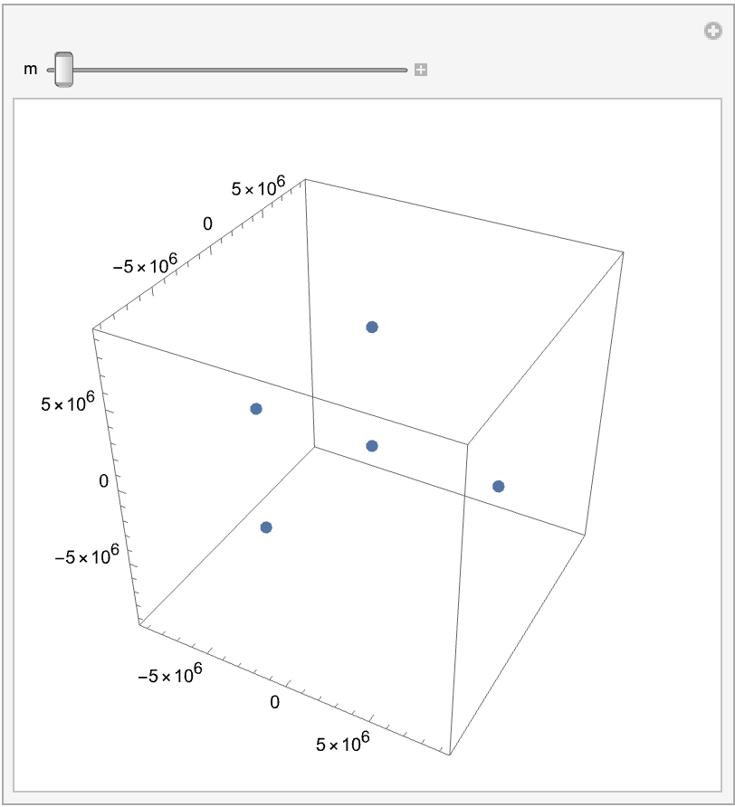
This is a manipulate function that shows frame by frame what happens in the simulation.
Uses manipulate to control the time t over the list of the positions:
In[]:=
Manipulate[ListPointPlot3D[fulllist[[m]],PlotRange->{{-earthRadius*1.5,earthRadius*1.5},{-earthRadius*1.5,earthRadius*1.5},{-earthRadius*1.5,earthRadius*1.5}},BoxRatios->{1,1,1}],{m,1,Length[fulllist],1}]
Out[]=
This is animated plot of the same thing as above.
In[]:=
ListAnimateTableShowListPointPlot3D[fulllist[[m]],PlotRange->{{-earthRadius*1.5,earthRadius*1.5},{-earthRadius*1.5,earthRadius*1.5},{-earthRadius*1.5,earthRadius*1.5}},BoxRatios->{1,1,1}],SphericalPlot3D5000000,{u,0,Pi},{v,0,2Pi},MeshNone,TextureCoordinateFunction({#5,1-#4}&),PlotStyleDirectiveSpecularity[White,10],Texture
,Lighting"Neutral",AxesFalse,RotationAction"Clip",Background->Black,{m,1,Length[fulllist],100}//Quiet
Out[]=
Future Works
Future Works
In the future, I want to track and determine where the satellites that fall out of orbit end up. Often during descent, the atmospheric drag and heat are so intense that many satellites and debris will completely burn up. But those that can survive pose a danger to people on Earth. Creating a system that tracks a satellite’s atmospheric burn-up or trajectory toward Earth would be very beneficial.
Additionally I could improve this program by implementing a randomness in how many satellites are created following a collision. Implementing an element of randomness following the collision is more realistic
Additionally I could improve this program by implementing a randomness in how many satellites are created following a collision. Implementing an element of randomness following the collision is more realistic
Applications
Applications
This system can be used to model all the current satellites in orbit of Earth. From there, future incidents can be determined and future launches of satellites can be modeled to see potential future collisions. This program can also be used in debris mitigation and the maneuvering of spacecrafts to avoid orbital debris.
Acknowledgements
Acknowledgements
I would like to thank my mentor Jack Madden for his support throughout this project. Additionally, I would like to all the TAs and the directors of the Wolfram High School Summer Research Program for providing this opportunity.
References
References
◼
Shikha Subramaniam, R. T. (2023, January 13). Space dodgers. The Washington Post. https://www.washingtonpost.com/technology/interactive/2023/space-debris-game/
◼
Garcia, M. (2015, April 14). Space debris and human spacecraft. NASA. https://www.nasa.gov/mission_pages/station/news/orbital_debris.html
◼
Wall, M. (2021, November 15). Kessler syndrome and the space debris problem. Space.com.
https://www.space.com/kessler-syndrome-space-debris
https://www.space.com/kessler-syndrome-space-debris
CITE THIS NOTEBOOK
CITE THIS NOTEBOOK
A system for modeling space debris collision
by Shubhan Bhattacharya
Wolfram Community, STAFF PICKS, July 13, 2023
https://community.wolfram.com/groups/-/m/t/2964631
by Shubhan Bhattacharya
Wolfram Community, STAFF PICKS, July 13, 2023
https://community.wolfram.com/groups/-/m/t/2964631