Abstract: Reconstructing 3D data from a single viewpoint in a fundamental human vision functionality is one of the most challenging tasks that most computer vision algorithms struggle with. In this project, we try to quantify and evaluate information content through entropy measure such that we obtain an optimal image, that could provide the maximum information for 3D reconstruction if we are constrained to make a reconstruction given one image. We try to explore if the entropy based calculations could be a good metric to reduce the number of images for image reconstruction. We calculated joint entropy between the difference of gray scale pixel intensities in horizontal and vertical directions of images of a 3D object, at different viewing positions and angles and choose the image with maximal entropy.
1.Introduction
1.Introduction
1.1 Motivation
1.1 Motivation
The reconstruction of 3D objects from images is an important task in the field of computer vision, medical image processing, and virtual reality. There exist both traditional and deep learning based reconstruction methods that have achieved remarkable results. In both cases, some algorithms reconstruct using a single image and multiple images as input. To reconstruct a 3D object from a single image require prior knowledge and assumptions, therefore, it is difficult to accomplish a good reconstruction from a real image. In general, 3D reconstruction from a single image is a challenging task as it is difficult to predict the invisible parts from a single image. In the following section, we briefly discuss two types of reconstruction techniques.
1.2 3D Reconstruction
1.2 3D Reconstruction
◼
Traditional Methods:
Traditional methods for 3D object reconstruction of a single image are often based on prior models or use 2D annotation. These methods are often limited to object reconstruction in a certain category. For example, assuming the illumination is fixed and the shape is restored from the shadow. Assuming surface smoothness, the shape is restored from the texture. Due to the complexity of the real datasets, this class of model requires assumptions that are less effective in real applications.
◼
Deep Learning based Methods:
With the continuous rise of deep learning in recent years, it has become pretty common to reconstruct 3D objects from a single 2D image by using deep neural networks. The 3D object reconstruction method based on deep learning is to train neural networks to learn the mapping relationship between 2D images and 3D objects. This is done by encoder decoder technique. The optimization involves a reconstructor that uses a 2D encoder and a 3D decoder. The reconstructor reconstructs a 3D shape from the input image. In the 2D encoder stage, input images are encoded into a latent space for feature compression. Convolutional Neural Net, ResNet, and Variational Auto Encoders (VAE) can be used for the encoding mode. Now this latent vector is converted into three-dimensional data by a 3D decoder. To generate 3D shapes from the input image, the entire network needs to combine low-level image features with higher-level part arrangement knowledge. Most 3D object reconstruction methods based on a single image choose to use low-level image features for this purpose.
In this project, we aim to quantify and evaluate information content through entropy measures to maximize the information content for 3D reconstruction from a single image.
1.3 Shannon’s Entropy in 2D
1.3 Shannon’s Entropy in 2D
Information entropy is the quantitative measure of the information transmitted by the image. The entropy H(X) of a discrete random variable X is defined by: H(X) = It is to be noted that, entropy doesn’t take into account the spatial information. For example the images shown below have the same entropy. Courtesy: https://stats.stackexchange.com/questions/235270/entropy-of-an-image
-p(x)logp(x)
∑
x⊂X
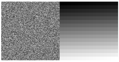
Lets take a look at the following example: Courtesy: https://stats.stackexchange.com/questions/235270/entropy-of-an-image
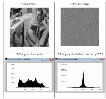
From the above figure, we see that, differential image has a more compact histogram. Therefore its information-entropy is higher. It is to be noted that, by definition entropy treats the intensity as the independent and identically distributed random variable .
Shannon defines different order of entropy corresponding to different approximations:
◼
Zeroth order approximation has all symbols independent and equi-probable.
◼
First order approximation has symbols independent with known probabilities.
◼
Second order approximation has symbol-pairs (diagrams) with known probabilities.
Both zeroth and first order entropies are isotropic and rotation invariant, but they are blind to any image structure. We therefore take the advantage of histogram shrinking property of finite difference operator.Joint entropy is defined as: H(▽f) =
J
-∑
j=1
I
∑
i=1
p
ij
log
2
p
ij
where is the joint probability of x derivative and y derivative component of a pixel in an image (in this context).
p
ij
2. Create Images from different point of views using Geometry3D
2. Create Images from different point of views using Geometry3D
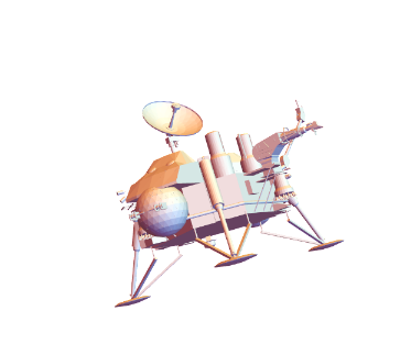
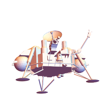
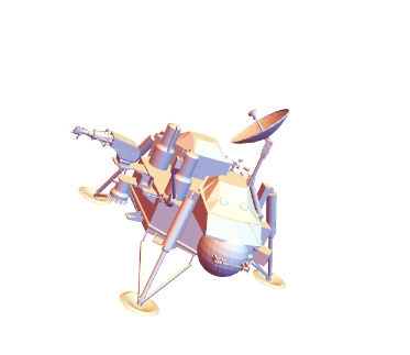
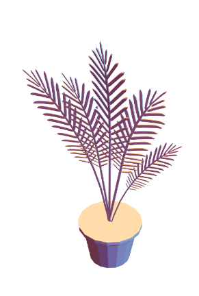
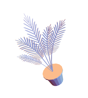
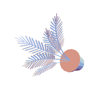
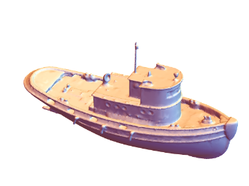
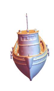
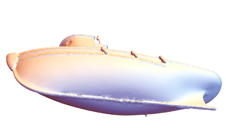
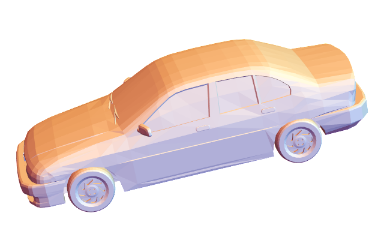
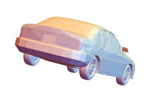
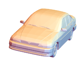
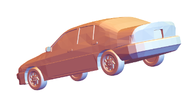
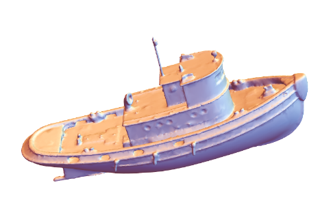
In order to create some synthetic source of image data, we take advantage of the inbuilt Mathematica function ‘Geometry3D’. We view the object from different view positions and view angles and then we rasterize it to create images. We have chosen 4 different objects, namely ‘VikingLander’, ‘PottedPlant’, ‘TugBoat’, ‘SedanCar’. Since we are trying to quantify the information content from a particular viewpoint, we choose a few positions simply ranging from more visual information to variably less. The specified view positions and angles are obtained by rasterizing as shown below.
◼
This function will give the rasterized image as the output along with view point and view angle at which it is rasterized.
In[]:=
ClearAll[getViewPointAndAngle](*getViewPointAndAngle[graphics3D_]:=Options[graphics3D,{ViewPoint,ViewAngle}]*)getViewPointAndAngle[graphics3D_]:=<|"Image"->Rasterize[graphics3D],Sequence@@Options[graphics3D,{ViewPoint,ViewAngle}]|>
In[]:=
ExampleData[{"Geometry3D","VikingLander"}]
Out[]=

In[]:=


Out[]=

Out[]=
Image
,ViewPoint{-0.958719,-3.08631,-1.00277}

In[]:=
association2= //getViewPointAndAngle
Out[]=
Image
,ViewPoint{-2.96428,-1.55247,-0.502861},ViewAngle0.350903
In[]:=
association3= //getViewPointAndAngle
Out[]=
Image
,ViewPoint{-0.725133,1.92674,-2.68549},ViewAngle0.350903

In[]:=
association4= //getViewPointAndAngle
Out[]=
Image
,ViewPoint{2.85986,-1.40641,1.13719},ViewAngle0.350903

◼
Summary of ‘VikingLander’ images and their corresponding view point and view angle.
In[]:=
vikinglanderImages=Merge[{association1,association2,association3,association4},Identity]
Out[]=
Image
,
,

,
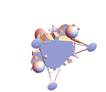
,ViewPoint{{-0.958719,-3.08631,-1.00277},{-2.96428,-1.55247,-0.502861},{-0.725133,1.92674,-2.68549},{2.85986,-1.40641,1.13719}},ViewAngle{0.350903,0.350903,0.350903}
In[]:=
ExampleData[{"Geometry3D","PottedPlant"}]
Out[]=

In[]:=
association5= //getViewPointAndAngle
Out[]=
Image
,ViewPoint{1.3,-2.4,2.},ViewAngleAutomatic

In[]:=
association6= //getViewPointAndAngle
Out[]=
Image
,ViewPoint{0.283961,2.56647,2.18692}

In[]:=
association7= //getViewPointAndAngle
Out[]=
Image
,ViewPoint{-0.255192,1.95439,2.7505}

In[]:=
association8= //getViewPointAndAngle
Out[]=
Image
,ViewPoint{-1.09786,-1.34158,2.90601}

◼
Summary of ‘PottedPlant’ images and their corresponding view point and view angle.
In[]:=
plantImages=Merge[{association5,association6,association7,association8},Identity]
Out[]=
Image
,
,
,
,ViewPoint{{1.3,-2.4,2.},{0.283961,2.56647,2.18692},{-0.255192,1.95439,2.7505},{-1.09786,-1.34158,2.90601}},ViewAngle{Automatic}

In[]:=
ExampleData[{"Geometry3D","Tugboat"}]
Out[]=

In[]:=
association9= //getViewPointAndAngle
Out[]=
Image
,ViewPoint{1.3,-2.4,2.},ViewAngleAutomatic
In[]:=
association10= //getViewPointAndAngle
Out[]=
Image
,ViewPoint{3.24986,0.141966,0.931797}
In[]:=
association11= //getViewPointAndAngle
Out[]=
Image
,ViewPoint{0.908624,1.87408,-2.66687}
In[]:=
association12= //getViewPointAndAngle
Out[]=
Image
,ViewPoint{0.548024,-2.80679,1.80876}

◼
Summary of ‘TugBoat’ images and their corresponding view point and view angle.
In[]:=
boatImages=Merge[{association9,association10,association11,association12},Identity]
Out[]=
Image
,

,

,

,ViewPoint{{1.3,-2.4,2.},{3.24986,0.141966,0.931797},{0.908624,1.87408,-2.66687},{0.548024,-2.80679,1.80876}},ViewAngle{Automatic}

In[]:=
ExampleData[{"Geometry3D","SedanCar"}]
Out[]=

In[]:=

Out[]=
In[]:=
association13= //getViewPointAndAngle
Out[]=
Image
,ViewPoint{0.880173,-3.14333,0.891509}

In[]:=
association14= //getViewPointAndAngle
Out[]=
Image
,ViewPoint{3.13019,-0.277471,1.25495}
In[]:=
association15= //getViewPointAndAngle
Out[]=
Image
,ViewPoint{2.44101,2.34142,-0.0959542}

In[]:=
association16=//getViewPointAndAngle
Out[]=
Image
,ViewPoint{-1.28831,3.12873,-0.0362937}
◼
Summary of ‘SedanCar’ images and their corresponding view point and view angle.
In[]:=
carImages=Merge[{association13,association14,association15,association16},Identity]
Out[]=
Image
,
,

,
,ViewPoint{{0.880173,-3.14333,0.891509},{3.13019,-0.277471,1.25495},{2.44101,2.34142,-0.0959542},{-1.28831,3.12873,-0.0362937}}

3. Entropy Calculation
3. Entropy Calculation
In the following section, we plot the gradient field vector of the rasterized images and calculate the entropy of each of them.
3.1 Gradient Field Vector Plot
3.1 Gradient Field Vector Plot
The following function takes in an image, convert it to grayscale and computes the gradient field based on the image gradient in horizontal and vertical directions. Later, it is plotted using ‘ListVectorPlot’.
In[]:=
ClearAll[ImageGradientField]ImageGradientField[image_]:=Module[{imageGray,gradientX,gradientY,gradientField,integerGradientField},imageGray=ColorConvert[image,"Grayscale"];gradientX=Differences[ImageData[imageGray],{0,1}];(*Echo[gradientX]*)gradientY=Differences[ImageData[imageGray],{1,0}];(*Echo[gradientY];*)gradientField=MapThread[List,{Most@gradientX,Transpose@Most@Transpose@gradientY},2];integerGradientField1=Round[gradientField*(256*256-1)];ListVectorPlot[Transpose[Reverse[integerGradientField1]],PlotRange->All]]
In[]:=
ImageGradientField
Out[]=
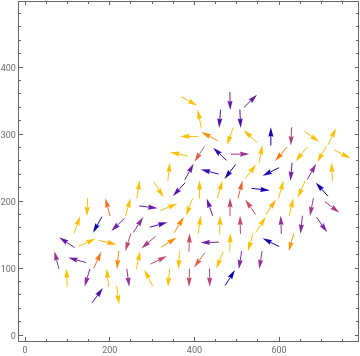
The gradient field of the ‘TugBoat’ and ‘SedanCar’ are plotted above using the ListVectorPlot. The gradient field of ‘VikingLander’ and ‘PottedPlant’ didn’t work out well, because of interpolation technique that the command internally is using.
3.2 Function for Entropy Calculation
3.2 Function for Entropy Calculation
The following function takes in an image and is used to compute the entropy of the image gradient gradient. Following are the steps involved:
◼
Convert the input image to gray scale image
◼
Compute the gradient in horizontal direction, i.e. find the difference between the consecutive pixels in horizontal direction.
◼
Compute the gradient in vertical direction, i.e. find the difference between the consecutive pixels in vertical direction.
◼
Scale the gradient field in order to get rid of fractional numbers
◼
Compute the entropy based on the joint probability distribution equation as above.
ClearAll[imageGradientEntropy]imageGradientEntropy[image_]:=Module[{imageGray,gradientX,gradientY,gradientField,gradientFieldScaled},imageGray=ColorConvert[image,"Grayscale"];gradientX=Differences[ImageData[imageGray],{0,1}];(*Echo[gradientX]*)gradientY=Differences[ImageData[imageGray],{1,0}];(*Echo[gradientY];*)gradientField=MapThread[List,{Most@gradientX,Transpose@Most@Transpose@gradientY},2];(*Echo[gradientField];*)gradientFieldScaled=Round[gradientField*(256*256-1)];(*Echo[gradientFieldScaled]*)Entropy@Flatten[gradientFieldScaled,1]//N]
In[]:=
{association1,association2,association3,association4}//Query[All,Append[#,<|"entropy"->imageGradientEntropy[#Image]|>]&]
Out[]=
Image
,ViewPoint{-0.958719,-3.08631,-1.00277},entropy1.19716,Image
,ViewPoint{-2.96428,-1.55247,-0.502861},ViewAngle0.350903,entropy0.911426,Image
,ViewPoint{-0.725133,1.92674,-2.68549},ViewAngle0.350903,entropy0.900846,Image
,ViewPoint{2.85986,-1.40641,1.13719},ViewAngle0.350903,entropy0.957626
In[]:=
{association5,association6,association7,association8}//Query[All,Append[#,<|"entropy"->imageGradientEntropy[#Image]|>]&]
Out[]=
Image
,ViewPoint{1.3,-2.4,2.},ViewAngleAutomatic,entropy1.21374,Image
,ViewPoint{0.283961,2.56647,2.18692},entropy0.886677,Image
,ViewPoint{-0.255192,1.95439,2.7505},entropy0.984043,Image
,ViewPoint{-1.09786,-1.34158,2.90601},entropy0.896206
In[]:=
{association9,association10,association11,association12}//Query[All,Append[#,<|"entropy"->imageGradientEntropy[#Image]|>]&]
Out[]=
Image
,ViewPoint{1.3,-2.4,2.},ViewAngleAutomatic,entropy2.18275,Image
,ViewPoint{3.24986,0.141966,0.931797},entropy2.28604,Image
,ViewPoint{0.908624,1.87408,-2.66687},entropy1.92751,Image
,ViewPoint{0.548024,-2.80679,1.80876},entropy2.50491
In[]:=
{association13,association14,association15,association16}//Query[All,Append[#,<|"entropy"->imageGradientEntropy[#Image]|>]&]
Out[]=
Image
,ViewPoint{0.880173,-3.14333,0.891509},entropy1.44197,Image
,ViewPoint{3.13019,-0.277471,1.25495},entropy1.36646,Image
,ViewPoint{2.44101,2.34142,-0.0959542},entropy1.37986,Image
,ViewPoint{-1.28831,3.12873,-0.0362937},entropy1.80756
3.3 Result
3.3 Result
It is evident from the above experiment, the image with more visual information has the highest entropy in the gradient field. It is clear from the VikingLander image-entropy comparison figure. It seems that the entropy of the image gradient field could be a promising metric for choosing an optimal image for 3D reconstruction.
4. Reconstruction using Commercial Tools
4. Reconstruction using Commercial Tools
In this section, we display the output when we use the maximum entropy images of ‘VikingLander’ as input to a commercial 3D reconstruction application, csm.ai.
In[]:=
lander1=Import[First@FileNames["vk1.mp4",FileNameJoin[{$HomeDirectory,"Downloads","RIT Wolfram seminar 4-2023","RIT Wolfram seminar 4-2023","Test Images"}]]]
Out[]=
In[]:=
lander2=Import[First@FileNames["vk2.mp4",FileNameJoin[{$HomeDirectory,"Downloads","RIT Wolfram seminar 4-2023","RIT Wolfram seminar 4-2023","Test Images"}]]]
Out[]=
In[]:=
GridVideo[{lander1,lander2}]
Out[]=
Clearly, the video in the right has lesser entropy and doesn’t catch much visual information. But generating 3D volume from single image is always challenging. Still it is doing pretty descent job.
5. Conclusion and Future Works
5. Conclusion and Future Works
In order to identify a metric that maximizes the information for 3D reconstruction from an image, we propose the use of Shannon’s entropy as a suitable metric. Furthermore, we explore its extension to reflect the structural complexity of the image. To conduct our study, we generated synthetic images by rasterizing selected objects from the ‘Geometry 3D’ dataset, varying the view position and angle. Subsequently, we calculated the joint entropy of the gradient field for these images, observing that images with more features exhibited higher entropy.
Based on our findings, we conclude that when faced with the task of selecting an image to maximize the information for 3D reconstruction, choosing the image with the highest entropy would be optimal. In future research, it would be valuable to delve deeper into implementing a 3D volumetric reconstruction framework in which we can use only the image with maximum entropy in the gradient field and compare its performance with state of art the Neural Radiance Field approach. The reconstruction should be such that we can rotate and see the reconstructed object from different viewpoints. This framework would specifically consider an image with maximum entropy as input.
Based on our findings, we conclude that when faced with the task of selecting an image to maximize the information for 3D reconstruction, choosing the image with the highest entropy would be optimal. In future research, it would be valuable to delve deeper into implementing a 3D volumetric reconstruction framework in which we can use only the image with maximum entropy in the gradient field and compare its performance with state of art the Neural Radiance Field approach. The reconstruction should be such that we can rotate and see the reconstructed object from different viewpoints. This framework would specifically consider an image with maximum entropy as input.
Keywords
Keywords
◼
Joint entropy
◼
Image gradient
◼
3D Reconstruction
Acknowledgment
Acknowledgment
First and foremost, I am deeply grateful to Stephen Wolfram for presenting me with an exciting problem statement to work on. I am sincerely grateful to my exceptional mentors, Sotiris Michos and Fez Zaman, for their unwavering guidance and support throughout this project.
I would also like to extend my heartfelt gratitude to Paul Abott and my doctoral advisor, Dr. Flip Phillips, for their generous technical insights towards my project. Additionally, I want to express my sincere thanks to our remarkable TA, Mark Greenberg, for diligently reviewing my work. I am also grateful to Mads Bahrami for exceptional coordination of the Summer School.
Together, these remarkable individuals, along with all the other members of WSS’23, have fostered an atmosphere of collaboration and synergy. I feel truly fortunate to have been surrounded by such a supportive and brilliant team. I am thankful to the entire team of WSS for providing me an amazing three weeks during the Summer.
References
References
◼
Kieran G. Larkin. Reflections on shannon information: In search of a natural information-entropy for images. CoRR, abs/1609.01117, 2016.
◼
Hanry Ham, Julian Wesley, and Hendra Hendra. Computer vision based 3d reconstruction: A review. International Journal of Electrical and Computer
Engineering, 9(4):2394, 2019.
Engineering, 9(4):2394, 2019.
◼
Kui Fu, Jiansheng Peng, Qiwen He, and Hanxiao Zhang. Single image 3d object reconstruction based on deep learning: A review. Multimedia Tools and Applications, 80:463–498, 2021
CITE THIS NOTEBOOK
CITE THIS NOTEBOOK
Quantifying an optimal image to maximize information for 3D reconstruction
by Tiyasa Sarkar
Wolfram Community, STAFF PICKS, July 12, 2023
https://community.wolfram.com/groups/-/m/t/2959398
by Tiyasa Sarkar
Wolfram Community, STAFF PICKS, July 12, 2023
https://community.wolfram.com/groups/-/m/t/2959398