Logistic growth model applied to the Covid-19 epidemic in Colombia
Diego Ramos
Universidad del Valle
Universidad del Valle
◼
This notebook is a computational essay using a package that can be downloaded at https://www.wolframcloud.com/obj/diego.ramos/Published/DatosCovidINS.wl.nb
◼
The package must be saved in the same directory as the notebook in order for it to be loaded automatically as part of initialization.
Methods
Methods
In this study we use the logistic function, first introduced in 1838 by the Belgian mathematician Verhulst and today with many applications in biology, epidemiology, statistics, machine learning, among other fields (see [2] and [3]). Verhulst introduced this function to model human populations under the thesis that in a territory of limited size and resources the number of inhabitants tends to stabilize at a maximum value that he called “carrying capacity” (see [1]). This model has been used in various biological populations and is known as the logistic growth model.
The logistic function is suitable for modeling many growth variables under environmental constraints. Just as population growth is limited by the size and resources of the territory, the spread of an epidemic can be limited through diagnostic systems and quarantine controls.
The logistic model can be expressed in the form of a logistic differential equation as
F
t
F(t)
L
t
0
L
2
(
1
)where , the cumulative count of individuals infected by COVID-19, is a function of time and can be expressed in terms of the parameters as the function Logistics
F(t)
β=(L,,k)
t
0
F(t)=.
L
1+
-k(t-)
t
0
(
2
)The parameter L represents the carrying capacity or maximum number of infections, represents the instant when or peak of the epidemic and k represents the relative growth rate o velocity of propagation.
t
0
F()=L/2
t
0
The duration of the epidemic, in days, is defined as the length of the time interval , where < and (véase [6]), and it can be expressed as
[,]
t
1
t
2
t
1
t
2
F'()=F'()=1
t
1
t
2
duracióndelaepidemia=Log
1
k
-2+2kL+
kL(-4+kL)
-2+2kL-
kL(-4+kL)
(
3
)Our purpose is to estimate the parameters using the non-linear least squares method. However, we will not estimate model (2) directly since previous studies indicate that deterministic models for the accumulated cases have a high serial correlation in terms of error, which generates imprecision in the parameter estimates (see [6] and [7]).Instead, the model we use to estimate the parameters is the derivative
β=(L,,k)
t
0
f(t,β)=F'(t)=,
kL
-k(t-)
t
0
2
(1+)
-k(t-)
t
0
(
4
)which allows us to model the daily count of new cases.
We denote by the probabilistic model of the daily count of new cases :
C
C=f(t,β)+ϵ
(
5
)We assume that the residual errors are independent and identically distributed random variables. With the non - linear least squares method we find the optimal parameter that minimizes the sum of the squares of the residual errors
ϵ
β
E(β)=.
∑
t
2
(C(t)-f(t,β))
(
6
)To do this we first provided adequate initial values of for the Levenberg-Marquart optimization algorithm to successfully converge to the global minimum of .
β
E(β)
The data
The data
Two sources were selected to make the model fit (4). One of these sources is the Johns Hopkins University (JHU), whose data is taken from the Wolfram Repository Data (WRD), which constitutes a public resource of organized and appropriate data sets for immediate use in computing, analysis, visualization, etc. . The second source is the National Institute of Health of Colombia (INS), which has made the registry of cases of contagion by Covid-19 available to the public.
The data in the Wolfram Repository Data is a dataset that has various information about the pandemic. We are only interested in obtaining the data from confirmed cases found in the ‘Confirmed Cases’ column of the dataset.
We retrieve data for counting cumulative cases in Colombia:
In[]:=
ResourceUpdate["Epidemic Data for Novel Coronavirus COVID-19"]//Quiet;ConteoAcumuladoUJH=ResourceData["Epidemic Data for Novel Coronavirus COVID-19","WorldCountries"][SelectFirst[#CountryEntity["Country","Colombia"]&],"ConfirmedCases"]
Out[]=
TimeSeries

From the accumulated count of cases, it is possible to obtain the daily count of new cases knowing the difference of each two consecutive accumulated data.
We obtain the daily count of new cases in Colombia in the time series format:
In[]:=
ConteoDiarioUJH=Differences[ConteoAcumuladoUJH]
Out[]=
TimeSeries
The National Institute of Health has provided a dataset with registration of confirmed cases and programmatic access via API Socrata Open Data (SODA); The data were chosen from the column ‘FIS’ (Symptom Onset Date) as prescribed by the INS at https://www.ins.gov.co/Noticias/Paginas/coronavirus-notas.aspx; For those who were asymptomatic, the corresponding data was assigned to the column ‘Notification Date’. A Wolfram code package was developed that contains a set of procedures to automate the access and curation of INS data which has been incorporated into the workflow of this computational assay. The package is named DataCovidINS.wl which has been loaded automatically from the initialization section.
We obtain the daily count of new cases in Colombia with the INS data:
In[]:=
ConteoDiarioINS=INSColombia[]
Out[]=
TimeSeries
From the daily count of cases it is possible to obtain the accumulated count by adding cumulatively.
We cumulatively add the daily cases to obtain the accumulated count:
In[]:=
ConteoAcumuladoINS=Accumulate[ConteoDiarioINS]
Out[]=
TimeSeries
When comparing the data provided by Wolfram Repository Data and the National Institute of Health, some discrepancies were observed, which led to the fitting of the model based on each of the data sources.
We graph the cumulative count based on each of the sources:
In[]:=
DateListPlot{ConteoAcumuladoINS,ConteoAcumuladoUJH},
Out[]=
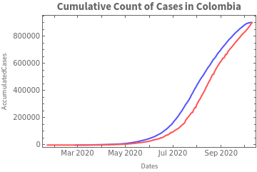
These differences led to the fitting of the model for each of the data sources.
Model fitting at the national level
Model fitting at the national level
In this section we propose to estimate the parameters of the model from the data obtained in the previous section. Once the model is estimated, we use the to estimate the date of the peak of the epidemic and with the parameters and we will estimate the duration of the epidemic, as well as the estimated date of the end of it.
t
0
k
L
Model fitting based on JHU data
Model fitting based on JHU data
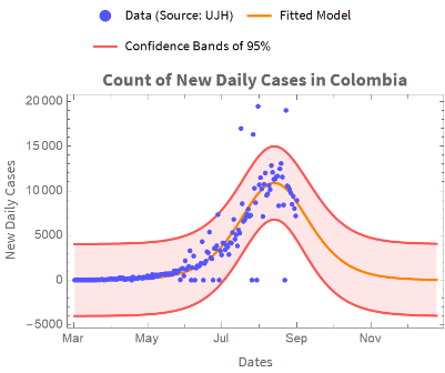
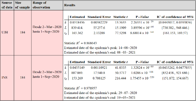
In what follows, we estimate model (4) from UJH data. The fit was made for the daily new case count from March 2, 2020 through September 1, 2020.
Nonlinear least squares model fitting with daily count data:
In[]:=
ColombiaModelDiariosUJH=NonlinearModelFitTimeSeriesWindow[ConteoDiarioUJH,{"2 Mar 2020","1 Sep 2020"}]["Values"],(kL),{{k,0.072},{L,907052.4},{t0,137.652}},t
-k(t-t0)
2
(1+)
-k(t-t0)
Out[]=
FittedModel
From the FittedModel object that we have just obtained, we can know the results and the diagnostics of the model. For now we are interested in the values of the estimated parameters.
From the FittedModel object that we have just obtained, we can know the results and the diagnostics of the model. For now we are interested in the values of the estimated parameters.
We extract the values of the estimated parameters of the fit:
In[]:=
ColombiaModelDiariosUJH["BestFitParameters"]
Out[]=
{k0.0518436,L839414.,t0165.362}
Since the peak of the epidemic occurs days after March 2 2020, we can obtain the estimated date of the peak of the epidemic by adding the date March 2, 2020 days.
t
0
t
0
We obtain the estimated date of the peak of the epidemic by adding days to 2 Mar 2020:
t
0
In[]:=
DateObject["2 Mar 2020"]+Quantity[t0/.ColombiaModelDiariosUJH["BestFitParameters"],"Days"]
Out[]=
In the Initialization section we have defined the duration variable that contains the formula that represents the duration of the epidemic. Replacing the estimates of the parameters in this formula we can obtain an estimate for the duration of the epidemic.
We replace the estimated values of the parameters and in the formula for the duration of the epidemic:
k
L
In[]:=
duracion/.ColombiaModelDiariosUJH["BestFitParameters"]
Out[]=
412.042
As can be seen [5] the estimate for the end of the epidemic, in days from the first recorded date, is given by
endofepidemic=peakday+(duracióndelaepidemia).
1
2
(
7
)From this result we can obtain an estimated date for the end of the epidemic in Colombia.
We replace the parameter estimates in equation (7) and add the days to March 2, 2020:
In[]:=
DateObject["2 Mar 2020"]+Quantity[(t0+1/2duracion)/.ColombiaModelDiariosUJH["BestFitParameters"],"Days"]
Out[]=
Let’s see a graphical representation of the results of the fit we have made.
We generate the confidence bands with a level of 0.95:
In[]:=
bandas95UJH=ColombiaModelDiariosUJH["SinglePredictionBands",ConfidenceLevel0.95];
The figure below represents the fitted model and the actual data along with the 0.95 level confidence bands.
We plot the actual data, the forecast data, and the confidence bands:
In[]:=
DateListPlotEvaluate@Join[{ColombiaModelDiariosUJH["Data"]},Transpose[Table[Flatten[{ColombiaModelDiariosUJH[t],bandas95UJH}],{t,115+Length[ColombiaModelDiariosUJH["Data"]]}]]],
Out[]=
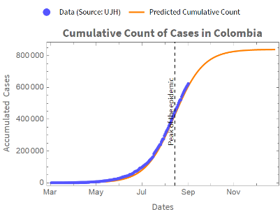
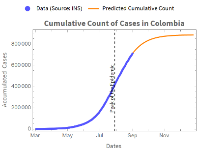
With the fitted model that we have obtained, we can forecast the accumulated count of cases.The following is a graph for the actual and predicted running count.
We obtain a plot of the accumulated cases from the estimated parameters and the accumulated count of cases:
In[]:=
DateListPlot{Accumulate@ColombiaModelDiariosUJH["Data"],Table[(L/(1+Exp[-k(#-t0)])/.ColombiaModelDiariosUJH["BestFitParameters"])&[t],{t,115+Length[ColombiaModelDiariosUJH["Data"]]}]},
Out[]=
Model fitting based on INS data
Model fitting based on INS data
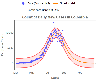
In what follows, we fit the model (4) to the data corresponding to the daily count of new cases, provided by the National Institute of Health. Estimate is based on data from March 2, 2020 through Sep 1, 2020.
Nonlinear least squares model fitting with daily count data:
In[]:=
ColombiaModelDiariosINS=NonlinearModelFitTimeSeriesWindow[ConteoDiarioINS,{"2 Mar 2020","1 Sep 2020"}]["Values"],(kL),{{k,0.07},{L,822612},{t0,158}},t
-k(t-t0)
2
(1+)
-k(t-t0)
Out[]=
FittedModel
From the FittedModel object that we have just obtained, we can know the results and diagnostics of the fit. For now we are interested in the values of the estimated parameters.
We extract the values of the parameter estimates:
In[]:=
ColombiaModelDiariosINS["BestFitParameters"]
Out[]=
{k0.0455149,L887069.,t0153.269}
We can use the estimated to estimate the date of the peak of the epidemic.
t
0
We add days to March 2 2020 to estimate the peak date of the epidemic:
t
0
In[]:=
DateObject["2 Mar 2020"]+Quantity[t0/.ColombiaModelDiariosINS["BestFitParameters"],"Days"]
Out[]=
Now we can estimate the duration of the epidemic, in days, by replacing the estimated values for the parameters in the variable duration.
We replace the estimated values of the parameters in the variable duration:
In[]:=
duracion/.ColombiaModelDiariosINS["BestFitParameters"]
Out[]=
466.042
This value gives us an estimate of the duration of the epidemic in Colombia. We can estimate the date of the end of the epidemic by replacing the estimated parameters in equation (7).
We add the corresponding days to March 2, 2020 to obtain the estimate of the end of the epidemic:
In[]:=
DateObject["2 Mar 2020"]+Quantity[(t0+1/2duracion)/.ColombiaModelDiariosINS["BestFitParameters"],"Days"]
Out[]=
We graphically represent the results of the fit we have made.
We can generate the confidence bands with a level of 0.95 by:
In[]:=
bandas95INS=ColombiaModelDiariosINS["SinglePredictionBands"];
We plot the actual data, the forecast data, and the confidence bands:
In[]:=
DateListPlotEvaluate@Join[{ColombiaModelDiariosINS["Data"]},Transpose[Table[Flatten[{ColombiaModelDiariosINS[t],bandas95INS}],{t,115+Length[ColombiaModelDiariosINS["Data"]]}]]],
Out[]=
With the fitted model that we have obtained, we can forecast the accumulated count of cases. Here is a chart for the actual and predicted cumulative count.
We obtain a graph of the accumulated cases from the model and the data of daily cases adding accumulatively:
In[]:=
DateListPlot{Accumulate@ColombiaModelDiariosINS["Data"],Table[(L/(1+Exp[-k(#-t0)])/.ColombiaModelDiariosINS["BestFitParameters"])&[t],{t,115+Length[ColombiaModelDiariosINS["Data"]]}]},
Out[]=
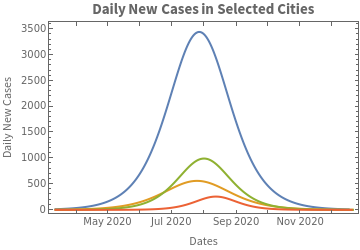
Model fitting for selected cities
Model fitting for selected cities
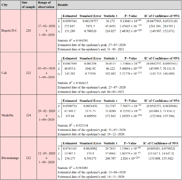
The cities Bogotá, Cali, Medellín and Bucaramanga were selected to fit the model (4). The DataCovidINS package provides the INSCiudad procedure to obtain the data corresponding to the daily count of new cases in the time series format. The procedure to make the fit to a specific city is the same as that made at the national level, which is why these adjustments are presented in the initialization section and below we only graphically show the results of such adjustment.
We plot on the same scale the curves that predict the daily count:
In[]:=
DateListPlot{Table[ModeloBogota[t],{t,14,110+Length[ModeloBogota["Data"]]}],Table[ModeloCali[t],{t,10,110+Length[ModeloCali["Data"]]}],Table[ModeloMedellin[t],{t,12,110+Length[ModeloMedellin["Data"]]}],Table[ModeloBucaramanga[t],{t,110+Length[ModeloBucaramanga["Data"]]}]},
Out[]=
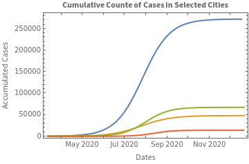
We graph on the same scale the logistic curves that predict the accumulated count of cases:
In[]:=
DateListPlot{Table[(L/(1+Exp[-k(#-t0)])/.ModeloBogota["BestFitParameters"])&[t],{t,14,110+Length[ModeloBogota["Data"]]}],Table[(L/(1+Exp[-k(#-t0)])/.ModeloCali["BestFitParameters"])&[t],{t,10,110+Length[ModeloCali["Data"]]}],Table[(L/(1+Exp[-k(#-t0)])/.ModeloMedellin["BestFitParameters"])&[t],{t,12,110+Length[ModeloMedellin["Data"]]}],Table[(L/(1+Exp[-k(#-t0)])/.ModeloBucaramanga["BestFitParameters"])&[t],{t,110+Length[ModeloBucaramanga["Data"]]}]},
Out[]=
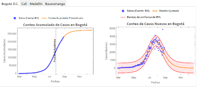
We present the results of each city in an interactive way :
Out[]=
Statistical analysis
Statistical analysis
The analysis at the national level is based on two different data sources : data from Johns Hopkins University and data from the National Institute of Health of Colombia.The same analysis was made for the cities Bogotá, Cali, Medellín and Bucaramanga based on the INS data only.
The results of fitting the model to the time series data corresponding to new cases of Covid-19 at the national level are shown:
Out[]=
The results of fitting the model to the time series data corresponding to new cases of Covid-19 at the selected cities:
Out[]=
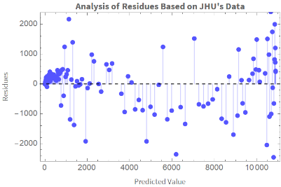
Residual analysis
Residual analysis
We plot the residuals vs the fitted values:
In[]:=
ListPlotTranspose[{Table[ColombiaModelDiariosUJH[t],{t,Length[ColombiaModelDiariosUJH["Data"]]}],ColombiaModelDiariosUJH["FitResiduals"]}],
Out[]=
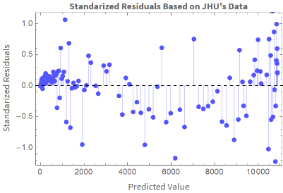
We plot the standardized residuals vs. the predicted values:
In[]:=
ListPlotTranspose[{Table[ColombiaModelDiariosUJH[t],{t,Length[ColombiaModelDiariosUJH["Data"]]}],ColombiaModelDiariosUJH["StandardizedResiduals"]}],
Out[]=
In[]:=
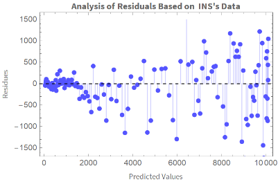
ListPlotTranspose[{Table[ColombiaModelDiariosINS[t],{t,Length[ColombiaModelDiariosINS["Data"]]}],ColombiaModelDiariosINS["FitResiduals"]}],
Out[]=
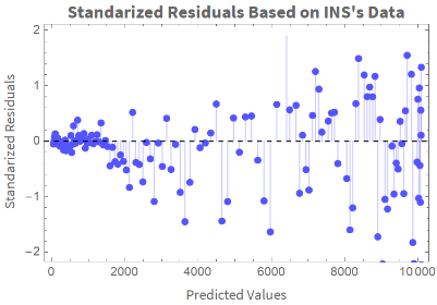
We plot the standardized residuals vs. the predicted values:
In[]:=
ListPlot[Transpose[{Table[ColombiaModelDiariosINS[t],{t,Length[ColombiaModelDiariosINS["Data"]]}],ColombiaModelDiariosINS["StandardizedResiduals"]}],AxesFalse,FrameTrue,PlotStyleLighter[Blue],FrameLabel{Style["Predicted Values","Text",12],Style["Standarized Residuals","Text",12]},PlotMarkersAutomatic,PlotLabelStyle["Standarized Residuals Based on INS's Data","Text",Bold],Epilog{Dashed,InfiniteLine[{{0,0},{1000,0}}]},FillingAxis]
Out[]=
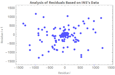
Graficamos el residuo i vs. el residuo i-1:
In[]:=
ListPlotTranspose[{ColombiaModelDiariosINS["FitResiduals"],RotateLeft@ColombiaModelDiariosINS["FitResiduals"]}],
Out[]=
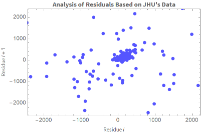
Graficamos el residuo i vs. el residuo i-1 :
In[]:=
ListPlotTranspose[{ColombiaModelDiariosUJH["FitResiduals"],RotateLeft@ColombiaModelDiariosUJH["FitResiduals"]}],
Out[]=
Analysis of variance
Analysis of variance
We obtain the analysis of variance for the model based on the UJH data:
In[]:=
TablaAnova[ColombiaModelDiariosUJH]
Out[]=
GL | RSS | MS | Estadístico F | Valor P | |
Mod. | 3 | 4.99318× 9 10 | 1.66439× 9 10 | 392.363 | 3.47553× -78 10 |
Error | 181 | 7.55071× 8 10 | 4.17166× 6 10 | ||
Tot. no Corr. | 184 | 5.74825× 9 10 | |||
Tot. Corr. | 183 | 3.6319× 9 10 |
We obtain the analysis of variance for the model based on the INS data:
In[]:=
TablaAnova[ColombiaModelDiariosINS]
Out[]=
GL | RSS | MS | Estadístico F | Valor P | |
Mod. | 3 | 5.38006× 9 10 | 1.79335× 9 10 | 2760.35 | 0. |
Error | 181 | 1.15643× 8 10 | 638914. | ||
Tot. no Corr. | 184 | 5.4957× 9 10 | |||
Tot. Corr. | 183 | 2.75169× 9 10 |
We obtain the analysis of variance for the model fitted for Bogota:
In[]:=
TablaAnova[ModeloBogota]
Out[]=
GL | RSS | MS | Estadístico F | Valor P | |
Mod. | 3 | 5.85619× 8 10 | 1.95206× 8 10 | 1867.16 | 0. |
Error | 181 | 1.86094× 7 10 | 102814. | ||
Tot. no Corr. | 184 | 6.04228× 8 10 | |||
Tot. Corr. | 183 | 3.16348× 8 10 |
We obtain the analysis of variance for the model fitted for Cali:
In[]:=
TablaAnova[ModeloCali]
Out[]=
GL | RSS | MS | Estadístico F | Valor P | |
Mod. | 3 | 1.70873× 7 10 | 5.69576× 6 10 | 1717.78 | 0. |
Error | 181 | 590207. | 3260.81 | ||
Tot. no Corr. | 184 | 1.76775× 7 10 | |||
Tot. Corr. | 183 | 8.2569× 6 10 |
We obtain the analysis of variance for the model fitted for Medellín:
In[]:=
TablaAnova[ModeloMedellin]
Out[]=
GL | RSS | MS | Estadístico F | Valor P | |
Mod. | 3 | 4.27119× 7 10 | 1.42373× 7 10 | 741.427 | 5.01776× -101 10 |
Error | 183 | 3.45646× 6 10 | 18887.8 | ||
Tot. no Corr. | 186 | 4.61684× 7 10 | |||
Tot. Corr. | 185 | 2.88462× 7 10 |
We obtain the analysis of variance for the model fitted for Bucaramanga:
In[]:=
TablaAnova[ModeloBucaramanga]
Out[]=
GL | RSS | MS | Estadístico F | Valor P | |
Mod. | 3 | 2.1818× 6 10 | 727266. | 1382.88 | 3.81788× -118 10 |
Error | 171 | 88352.6 | 516.682 | ||
Tot. no Corr. | 174 | 2.27015× 6 10 | |||
Tot. Corr. | 173 | 1.55501× 6 10 |
Key words
Key words
◼
Logistic Function
◼
Covid-19
◼
Nonlinear least squares method
References
References
[1] Bacaër N. " A Short Historory of Mathematical Population Dynamics". Springer - Verlag, 2010
[2] Dmitry Kucharavy, Roland De Guio. "Application of Logistic Growth Curve". ELSEVIER, 2015.
[4] Robert Rimmer. "Logistic Model For Quarentine Controled Epidemics", https://community.wolfram.com/groups/-/m/t/1900530
[5] Mads Bahrami y Brian Wood. "Logistic Model for COVID-19", https://www.wolframcloud.com/obj/covid-19/Published/Logistic-Growth-Model-for-COVID-19.nb
[6] Aaron A. King, Matthieu Domenech de Celle‘s, Felicia M. G. Magpantay1 and Pejman Rohani. “Avoidable errors in the modelling of outbreaks of emerging pathogens, with special
reference to Ebola”, 2015.
reference to Ebola”, 2015.
[7] Christopher Y. Shen. “Logistic growth modelling of COVID-19 proliferation in China and its in ternational implications”. ELSEVIER, 2020.
Inicialization
Inicialization
Load the package DatosCovidINS:
In[]:=
SetDirectory[NotebookDirectory[]];Get["DatosCovidINS.wl"]
Usage of INSCiudad:
In[]:=
?INSCiudad
Out[]=
Usage of INSColombia:
In[]:=
?INSColombia
Out[]=
we define the variable duration:
In[]:=
duracion=(1/k)Log-2+kL+√(kL(-4+kL))-2+kL-√(kL(-4+kL));
Fit the model for Bogotá
In[]:=
BogotaConteoDiario=INSCiudad["Bogotá D.C."];ModeloBogota=NonlinearModelFitTimeSeriesWindow[BogotaConteoDiario,{DateObject["2 Mar 2020"],"1 Sep 2020"}]["Values"],(kL),{{k,0.05},{L,182262},{t0,108}},t;BandasBogota=ModeloBogota["SinglePredictionBands"];
-k(t-t0)
2
(1+)
-k(t-t0)
Fit the model for Cali
In[]:=
CaliConteoDiario=INSCiudad["Cali"];ModeloCali=NonlinearModelFitTimeSeriesWindow[CaliConteoDiario,{CaliConteoDiario["FirstDate"],"1 Sep 2020"}]["Values"],(kL),{{k,0.05},{L,52262},{t0,108}},t;BandasCali=ModeloCali["SinglePredictionBands"];
-k(t-t0)
2
(1+)
-k(t-t0)
fit the model for Medellin:
In[]:=
MedellinConteoDiario=INSCiudad["Medellín"];ModeloMedellin=NonlinearModelFitTimeSeriesWindow[MedellinConteoDiario,{MedellinConteoDiario["FirstDate"],"1 Sep 2020"}]["Values"],(kL),{{k,0.05},{L,52262},{t0,108}},t;BandasMedellin=ModeloMedellin["SinglePredictionBands"];
-k(t-t0)
2
(1+)
-k(t-t0)
fit the model for Bucaramanga:
In[]:=
BucaramangaConteoDiario=INSCiudad["Bucaramanga"];ModeloBucaramanga=NonlinearModelFitTimeSeriesWindow[BucaramangaConteoDiario,{BucaramangaConteoDiario["FirstDate"],"1 Sep 2020"}]["Values"],(kL),{{k,0.05},{L,5222},{t0,88}},t;BandasBucaramanga=ModeloBucaramanga["SinglePredictionBands"];
-k(t-t0)
2
(1+)
-k(t-t0)
In[]:=
TablaAnova[model_]:=With[{AnovaEntradas=model["ANOVATableEntries"]},Grid[Join[{{"","GL","RSS","MS","Estadístico F","Valor P"}},Transpose@Join[{{"Mod.","Error","Tot. no Corr.","Tot. Corr."}},Transpose[PadRight[#,3,""]&/@AnovaEntradas],{{(AnovaEntradas[[1,2]]/3)/(AnovaEntradas[[2,2]]/(model["ANOVATableDegreesOfFreedom"][[2]]-3)),"","",""}},{{NProbability[F>(AnovaEntradas[[1,2]]/3)/(AnovaEntradas[[2,2]]/(model["ANOVATableDegreesOfFreedom"][[2]]-3)),FFRatioDistribution[3,model["ANOVATableDegreesOfFreedom"][[2]]-3]]//Quiet,"","",""}}]],FrameAll,BaseStyle{FontFamily"Times New Roman"},Background{False,{LightGray},{{{2,5},{1,1}}LightRed}}]]